Statistics, Science, Random Ramblings
A blog about data and other interesting things
An introduction to tidymodels
Recently, the tidymodels family of packages has gained some attention,
although some of the included packages have been around for a while.
However, as of February 2020 many of the involved packages still have a version
number of 0.0.x, so it is likely that things will change quite a bit in
the future.
What is tidymodels?
What the tidyverse family of packages is for data wrangling, the
tidymodels
family aims to be for modelling.
Additionally, what scikit-learn is for Python, tidymodels could be for R.
There are numerous packages available that implement various kinds of
modelling and predicting data available in R, all with their own
properties, quirks and features.
This is where tidymodels comes in, as it provides a standardised interface
to various modelling packages, so modelling and predicting becomes a
straightforward process.
In this blog post I will go through several steps of using tidymodels from
data preprocessing to hyperparameter tuning.
The data used is a dataset on bike rentals in Washington D.C., USA in 2011 and 2012.
If you want to skip the data exploration and data wrangling part below, click here to jump directly to the preprocessing section.
Data exploration
Load the required packages and set a seed for reproducibility.
Similar as with tidyverse, calling library("tidymodels") will load many
packages at once.
library("tidyverse")
library("tidymodels")
set.seed(4757)
Of course, first we should read the data set.
bikes <- read_csv("bikes_hour.csv")And now have a look at it.
glimpse(bikes)## Observations: 17,379
## Variables: 17
## $ instant <dbl> 1, 2, 3, 4, 5, 6, 7, 8, 9, 10, 11, 12, 13, 14, 15, 16, 17,…
## $ dteday <date> 2011-01-01, 2011-01-01, 2011-01-01, 2011-01-01, 2011-01-0…
## $ season <dbl> 1, 1, 1, 1, 1, 1, 1, 1, 1, 1, 1, 1, 1, 1, 1, 1, 1, 1, 1, 1…
## $ yr <dbl> 0, 0, 0, 0, 0, 0, 0, 0, 0, 0, 0, 0, 0, 0, 0, 0, 0, 0, 0, 0…
## $ mnth <dbl> 1, 1, 1, 1, 1, 1, 1, 1, 1, 1, 1, 1, 1, 1, 1, 1, 1, 1, 1, 1…
## $ hr <dbl> 0, 1, 2, 3, 4, 5, 6, 7, 8, 9, 10, 11, 12, 13, 14, 15, 16, …
## $ holiday <dbl> 0, 0, 0, 0, 0, 0, 0, 0, 0, 0, 0, 0, 0, 0, 0, 0, 0, 0, 0, 0…
## $ weekday <dbl> 6, 6, 6, 6, 6, 6, 6, 6, 6, 6, 6, 6, 6, 6, 6, 6, 6, 6, 6, 6…
## $ workingday <dbl> 0, 0, 0, 0, 0, 0, 0, 0, 0, 0, 0, 0, 0, 0, 0, 0, 0, 0, 0, 0…
## $ weathersit <dbl> 1, 1, 1, 1, 1, 2, 1, 1, 1, 1, 1, 1, 1, 2, 2, 2, 2, 2, 3, 3…
## $ temp <dbl> 0.24, 0.22, 0.22, 0.24, 0.24, 0.24, 0.22, 0.20, 0.24, 0.32…
## $ atemp <dbl> 0.2879, 0.2727, 0.2727, 0.2879, 0.2879, 0.2576, 0.2727, 0.…
## $ hum <dbl> 0.81, 0.80, 0.80, 0.75, 0.75, 0.75, 0.80, 0.86, 0.75, 0.76…
## $ windspeed <dbl> 0.0000, 0.0000, 0.0000, 0.0000, 0.0000, 0.0896, 0.0000, 0.…
## $ casual <dbl> 3, 8, 5, 3, 0, 0, 2, 1, 1, 8, 12, 26, 29, 47, 35, 40, 41, …
## $ registered <dbl> 13, 32, 27, 10, 1, 1, 0, 2, 7, 6, 24, 30, 55, 47, 71, 70, …
## $ cnt <dbl> 16, 40, 32, 13, 1, 1, 2, 3, 8, 14, 36, 56, 84, 94, 106, 11…There are the following columns:
- instant: a unique id for each record
- dteday: the date of the record
- season: 1 to 4, spring to winter
- yr, mnth, hr: year, month, hour
- holiday, weekday, workingday: whether it is a holiday, weekday or working day
- weathersit: 1 to 4, with 1 being clear weather and 4 heavy precipitation
- temp, atemp: temperature and feels-like temperature, divided by the maximum for each variable
- hum: relative humidity divided by 100 (the maximum)
- windspeed: windspeed divided by 67 (the maximum), unit is unclear but sounds like mph
- casual, registered, cnt: amount of rentals by casual/registered/total users
Are there missings?
sum(is.na(bikes))## [1] 0No missings, that’s always nice. Let’s further look whether something in the data seems off:
summary(bikes)## instant dteday season yr
## Min. : 1 Min. :2011-01-01 Min. :1.000 Min. :0.0000
## 1st Qu.: 4346 1st Qu.:2011-07-04 1st Qu.:2.000 1st Qu.:0.0000
## Median : 8690 Median :2012-01-02 Median :3.000 Median :1.0000
## Mean : 8690 Mean :2012-01-02 Mean :2.502 Mean :0.5026
## 3rd Qu.:13034 3rd Qu.:2012-07-02 3rd Qu.:3.000 3rd Qu.:1.0000
## Max. :17379 Max. :2012-12-31 Max. :4.000 Max. :1.0000
## mnth hr holiday weekday
## Min. : 1.000 Min. : 0.00 Min. :0.00000 Min. :0.000
## 1st Qu.: 4.000 1st Qu.: 6.00 1st Qu.:0.00000 1st Qu.:1.000
## Median : 7.000 Median :12.00 Median :0.00000 Median :3.000
## Mean : 6.538 Mean :11.55 Mean :0.02877 Mean :3.004
## 3rd Qu.:10.000 3rd Qu.:18.00 3rd Qu.:0.00000 3rd Qu.:5.000
## Max. :12.000 Max. :23.00 Max. :1.00000 Max. :6.000
## workingday weathersit temp atemp
## Min. :0.0000 Min. :1.000 Min. :0.020 Min. :0.0000
## 1st Qu.:0.0000 1st Qu.:1.000 1st Qu.:0.340 1st Qu.:0.3333
## Median :1.0000 Median :1.000 Median :0.500 Median :0.4848
## Mean :0.6827 Mean :1.425 Mean :0.497 Mean :0.4758
## 3rd Qu.:1.0000 3rd Qu.:2.000 3rd Qu.:0.660 3rd Qu.:0.6212
## Max. :1.0000 Max. :4.000 Max. :1.000 Max. :1.0000
## hum windspeed casual registered
## Min. :0.0000 Min. :0.0000 Min. : 0.00 Min. : 0.0
## 1st Qu.:0.4800 1st Qu.:0.1045 1st Qu.: 4.00 1st Qu.: 34.0
## Median :0.6300 Median :0.1940 Median : 17.00 Median :115.0
## Mean :0.6272 Mean :0.1901 Mean : 35.68 Mean :153.8
## 3rd Qu.:0.7800 3rd Qu.:0.2537 3rd Qu.: 48.00 3rd Qu.:220.0
## Max. :1.0000 Max. :0.8507 Max. :367.00 Max. :886.0
## cnt
## Min. : 1.0
## 1st Qu.: 40.0
## Median :142.0
## Mean :189.5
## 3rd Qu.:281.0
## Max. :977.0Based on the information from summary, there are no obvious issues.
Let’s also visually explore the data:
bikes %>%
    select(-instant, -dteday) %>%
    pivot_longer(everything()) %>%
    ggplot() +
        aes(x = value) +
        geom_density() +
        facet_wrap(~name, scales = "free")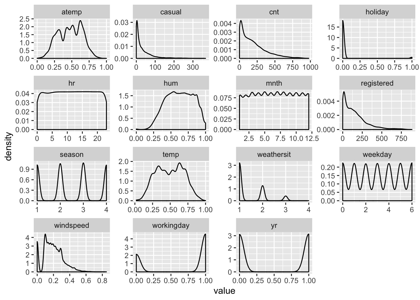
There are two things we can see here:
- Some variables should be turned into factors, because while using
numbers to represent their value, they are not continuous. In most cases this
was already obvious from the description of the data, but we got a nice visual
confirmation here. This is the case for variables like
seasonorweekdaywith many clear defined peaks in the data distribution. - Windspeed has a suspicious peak at 0.
Let’s have a closer look at windspeed:
bikes %>%
    select(windspeed) %>%
    ggplot() +
        aes(x = windspeed) +
        geom_histogram(binwidth = 0.05)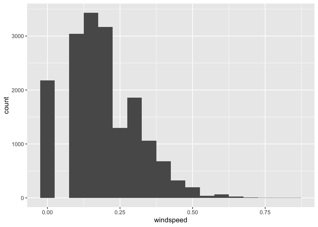
There is an unexpected amount of 0 values in the data. It is difficult to say why this is the case, but likely those are essentially missings. Dropping the column might be reasonable.
Now, let’s take a closer look at our dependent variable: the amount of bikes rented:
bikes %>%
    select(dteday, cnt, casual, registered) %>%
    pivot_longer(-dteday) %>%
    ggplot() +
        aes(x = dteday, y = value) +
        geom_line() +
        facet_grid(name~.)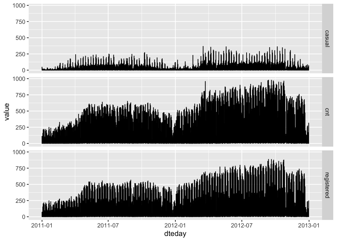
There is an obvious trend in the data for more rented bikes in 2012 compared to 2011. Under normal circumstances we should probably address that. Things we could do here are time series modelling and/or normalising our data by the total amount of registered users - if we were running a bike sharing business we should have that information available. However, this issue is beyond the scope of this post.
We will drop the casual and registered columns, as both are
included in cnt.
We can confirm this easily:
all(bikes$casual + bikes$registered == bikes$cnt)## [1] TRUETo finish the exploration we should also have a look at correlations between variables to identify pairs of highly correlated variables and also to get an idea of which predictors might be related to our dependent variable.
bikes %>%
    select(-instant, -dteday) %>%
    cor() %>%
    as_tibble(rownames = "x") %>%
    pivot_longer(-x) %>%
    ggplot() +
        aes(x = x, y = name, fill = value) +
        geom_raster() +
        scale_fill_gradient2(low = "purple", mid = "white",
                             high = "orangered") +
        labs(x = NULL, y = NULL) +
        theme(axis.text.x = element_text(
            angle = 90, hjust = 1, vjust = 0.5))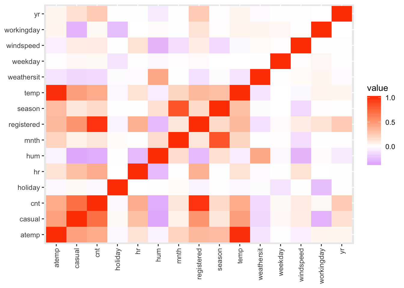
From the correlation heat map we can see that temp and atemp are
unsurprisingly highly correlated.
Furthermore cnt appears to be to some extend correlated with time of the day
and variables on weather conditions like temp and humidity.
So, after exploring the data, we will try dropping the
windpseed column as it contains a suspicious amount of 0 values, as well
as the casual and registered columns as we are only interested in the
total amount if bikes rented.
The temp and atemp variables are highly correlated, so we should remove
one of them, but to explore tidymodels we will keep them for now and set up a
preprocessing that handles those.
bikes2 <- bikes %>%
    select(-casual, -registered, -windspeed)
We will also remove the year variable as we saw in the plot above that in
2012 much more bikes were rented than in 2011.
While not exactly the best approach, as touched upon above,
it should do well enough for demonstrating tidymodels.
bikes2 <- bikes2 %>% select(-yr)As hr is discrete in our data and we will later dummy code our
variables, we will try to reduce its levels here.
bikes2 <- bikes2 %>%
  mutate(hr_cat = as_factor(hr)) %>%
  mutate(hr_cat = fct_collapse(.$hr_cat,
    "night" = as.character(c(0:6)),
    "morning" = as.character(c(7:12)),
    "afternoon" = as.character(c(13:18)),
    "evening" = as.character(c(19:23))
  )) %>%
  select(-hr)
Finally, we turn discrete variables into factors:
bikes2 <- bikes2 %>%
  mutate_at(vars(season, mnth, holiday, weekday,
                 workingday, weathersit), as_factor)
Preprocessing with tidymodels
The next thing you probably want to do is splitting the data into
test and train dataset.
We shuffle the rows of the dataset to not split at a
time point when we divide the data.
The default with sample_frac in dplyr is that it samples 100% of the
data without replacement, giving a nice tool for quick shuffling of rows.
bikes2 <- sample_frac(bikes2)We first prepare the split by calling initial_split from the rsample
package from the tidymodels family.
Here, we theoretically could add stratified splitting and of course set
the amount of data to put into each split, but the default of using 75% of
data is a sane choice.
bike_split <- initial_split(bikes2)
bike_split
## <13035/4344/17379>The initial_split function returns a rset object defining the split,
but not carrying it out yet.
Next, we extract our actual train and test datasets, which turn out to be tibbles.
bike_train <- training(bike_split)
bike_test <- testing(bike_split)
bike_train
## # A tibble: 13,035 x 13
## instant dteday season mnth holiday weekday workingday weathersit temp
## <dbl> <date> <fct> <fct> <fct> <fct> <fct> <fct> <dbl>
## 1 3479 2011-05-29 2 5 0 0 0 1 0.7
## 2 7754 2011-11-24 4 11 1 4 0 1 0.5
## 3 8811 2012-01-07 1 1 0 6 0 1 0.44
## 4 9028 2012-01-17 1 1 0 2 1 2 0.26
## 5 13832 2012-08-04 3 8 0 6 0 1 0.86
## 6 7776 2011-11-25 4 11 0 5 1 1 0.52
## 7 5503 2011-08-22 3 8 0 1 1 1 0.68
## 8 5836 2011-09-05 3 9 1 1 0 1 0.74
## 9 8925 2012-01-12 1 1 0 4 1 1 0.46
## 10 4601 2011-07-15 3 7 0 5 1 1 0.7
## # … with 13,025 more rows, and 4 more variables: atemp <dbl>, hum <dbl>,
## # cnt <dbl>, hr_cat <fct>Depending on the data and the methods you use, you often need to do some kind of
preprocessing.
This usually involves removal of highly correlated variables, dummy coding as well as scaling and centring of the data.
Tidymodels allows you to define a pipeline for preprocessing you can then
apply to the data, using tools from the recipes package.
To do so you first define what kind of variables you have:
base_recipe <- recipe(x = bike_train) %>%
  update_role(everything(), new_role = "predictor") %>%
  update_role(instant, dteday, new_role = "idvar") %>%
  update_role(cnt, new_role = "outcome")
Here we added roles to the variables in our data. This allows us to specify what we want to do with the data in our preprocessing pipeline as for everything we do in there we can define to which roles and variable types the steps should be applied.
We can choose the names of our roles pretty much the way we like
them, however there are selection functions for predictor so you
might want to use that role for your predictors.
What roles do should become clearer when we build and apply our pipeline.
pipeline <- base_recipe %>%
  step_nzv(all_predictors()) %>%
  step_knnimpute(all_predictors()) %>%
  step_center(all_numeric(), -has_role("outcome"),  -has_role("idvar")) %>%
  step_scale(all_numeric(), -has_role("outcome"),  -has_role("idvar")) %>%
  step_dummy(all_predictors(), -all_numeric()) %>%
  step_corr(all_numeric(), -has_role("outcome"),  -has_role("idvar"),
            threshold = 0.9)
Here we remove data with near zero variance, impute missing values using k-Nearest-Neighbours (there are no missings in our data, but I included this step for demonstrating it), dummy code categorical variables, centre and scale and finally remove variables if they highly correlate with another.
Using selector functions we specify to which role or type each step should
be applied. With all_predictors we choose everything that has the role
predictor, while with has_role we can select specific roles.
If a - is added before a selector we exclude that type or role, allowing
us to easily specify the set of variables we want a step to be applied to.
Our defined preprocessing pipeline can then be initialised, which does the estimation of parameters for the steps.
pipeline_prep <- prep(pipeline, training = bike_train,
                      strings_as_factors = FALSE)
We can also inspect the object to get some more information about the
steps.
For example we can see that the holiday column will be removed due to it
having almost no variance and temp will be removed due to it being highly
correlated with another variable (most likely atemp).
pipeline_prep## Data Recipe
##
## Inputs:
##
## role #variables
## idvar 2
## outcome 1
## predictor 10
##
## Training data contained 13035 data points and no missing data.
##
## Operations:
##
## Sparse, unbalanced variable filter removed holiday [trained]
## K-nearest neighbor imputation for mnth, weekday, workingday, weathersit, ... [trained]
## Centering for temp, atemp, hum [trained]
## Scaling for temp, atemp, hum [trained]
## Dummy variables from season, mnth, weekday, workingday, weathersit, hr_cat [trained]
## Correlation filter removed temp [trained]And then we apply it to the data.
training <- bake(pipeline_prep, new_data = bike_train)
testing <- bake(pipeline_prep, new_data = bike_test)
Our training dataset now looks like this:
training## # A tibble: 13,035 x 32
## instant dteday atemp hum cnt season_X2 season_X3 season_X4
## <dbl> <date> <dbl> <dbl> <dbl> <dbl> <dbl> <dbl>
## 1 3479 2011-05-29 1.12 0.846 219 1 0 0
## 2 7754 2011-11-24 0.0603 -1.48 114 0 0 1
## 3 8811 2012-01-07 -0.204 -1.27 109 0 0 0
## 4 9028 2012-01-17 -1.44 0.381 12 0 0 0
## 5 13832 2012-08-04 1.83 -1.17 547 0 1 0
## 6 7776 2011-11-25 0.149 -1.22 272 0 0 1
## 7 5503 2011-08-22 0.943 0.122 12 0 1 0
## 8 5836 2011-09-05 1.30 0.381 357 0 1 0
## 9 8925 2012-01-12 -0.116 0.0188 495 0 0 0
## 10 4601 2011-07-15 1.03 -0.602 265 0 1 0
## # … with 13,025 more rows, and 24 more variables: mnth_X2 <dbl>, mnth_X3 <dbl>,
## # mnth_X4 <dbl>, mnth_X5 <dbl>, mnth_X6 <dbl>, mnth_X7 <dbl>, mnth_X8 <dbl>,
## # mnth_X9 <dbl>, mnth_X10 <dbl>, mnth_X11 <dbl>, mnth_X12 <dbl>,
## # weekday_X1 <dbl>, weekday_X2 <dbl>, weekday_X3 <dbl>, weekday_X4 <dbl>,
## # weekday_X5 <dbl>, weekday_X6 <dbl>, workingday_X1 <dbl>,
## # weathersit_X2 <dbl>, weathersit_X3 <dbl>, weathersit_X4 <dbl>,
## # hr_cat_morning <dbl>, hr_cat_afternoon <dbl>, hr_cat_evening <dbl>Under normal circumstances we should have dropped the idvar and dteday
columns beforehand, but I wanted to demonstrate the use of roles in
preprocessing with tidymodels and thus left them in.
training <- training %>%
  select(-instant, -dteday)
Building and evaluating a model
Linear Regression
First, we go with a simple approach. When modelling the first thing you try should almost always be a linear model, so let’s build one:
lmod <- linear_reg() %>%
  set_engine("lm")
When using tidymodels you create a model object and select an engine
which it should use before fitting and predicting (to be more specific:
those functions are provided by the parsnip package).
In the case above we say that we want a linear regression
using lm.
Now, what’s the difference to just calling lm directly?
It is the workflow: for a single model family seen in isolation it does not
matter much, but when using several different model families you are quickly
confronted with slight differences in using them.
tidymodels however, enables you to use the exact same workflow for various
kinds of models without having to worry about differences between different
packages.
We can fit our model by passing it into the fit function and specifying the
formula we want to use.
lmod_fit <- lmod %>% fit(training, formula = cnt ~ .)And now we can make predictions. You can just pass the model into the predict
function if you like, but here we want to combine the predictions with the data, so we will opt for a slightly more complex construction with mutate.
training2 <- training %>%
  mutate(lm_pred = lmod_fit %>%
           predict(training) %>%
           deframe())
testing <- testing %>%
  mutate(lm_pred = lmod_fit %>%
           predict(testing) %>%
           deframe())
Using the metrics function from the yardstick package we can get some
metrics about how good our predictions are.
First we check on the training data.
training2 %>% metrics(cnt, lm_pred)## # A tibble: 3 x 3
## .metric .estimator .estimate
## <chr> <chr> <dbl>
## 1 rmse standard 129.
## 2 rsq standard 0.500
## 3 mae standard 95.3And now on the test data.
testing %>% metrics(cnt, lm_pred)## # A tibble: 3 x 3
## .metric .estimator .estimate
## <chr> <chr> <dbl>
## 1 rmse standard 128.
## 2 rsq standard 0.495
## 3 mae standard 94.0Errors on train and test data are similar, suggesting that there is no overfitting.
To evaluate how well our model does work we can of course plot the predicted data against the actual data:
ggplot(testing) +
  aes(x = cnt, y = lm_pred) +
  geom_abline(intercept = 0, slope = 1) +
geom_point(alpha = .5) 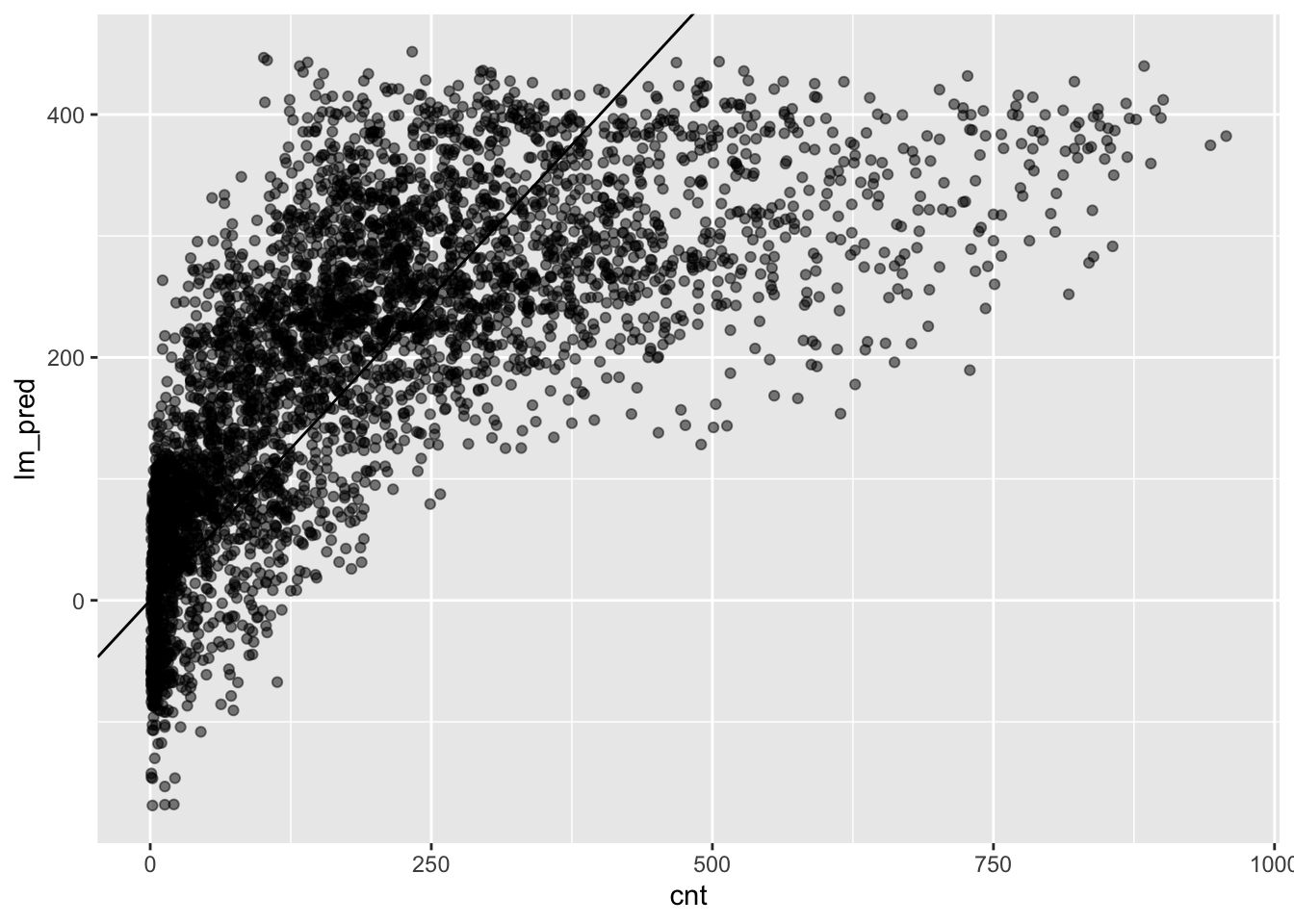
The plot does not exactly suggest that our predictive performance is good.
There are two obvious issues: 1. we predict values below 0 which does not
make sense given the data; 2. we have really large prediction errors for large
values of cnt.
You might also wonder how you access the underlying lm object. Well, this
is easy:
ls(lmod_fit)## [1] "elapsed" "fit" "lvl" "preproc" "spec"The actual model is contained in the fit.
summary(lmod_fit$fit)##
## Call:
## stats::lm(formula = formula, data = data)
##
## Residuals:
## Min 1Q Median 3Q Max
## -330.15 -80.56 -22.76 58.11 584.68
##
## Coefficients:
## Estimate Std. Error t value Pr(>|t|)
## (Intercept) 7.317 6.491 1.127 0.259697
## atemp 45.477 2.371 19.177 < 2e-16 ***
## hum -18.518 1.461 -12.672 < 2e-16 ***
## season_X2 42.530 7.096 5.993 2.11e-09 ***
## season_X3 33.197 8.475 3.917 9.01e-05 ***
## season_X4 69.134 7.125 9.704 < 2e-16 ***
## mnth_X2 5.418 5.681 0.954 0.340273
## mnth_X3 9.758 6.345 1.538 0.124107
## mnth_X4 -2.812 9.459 -0.297 0.766221
## mnth_X5 19.435 10.014 1.941 0.052313 .
## mnth_X6 2.682 10.137 0.265 0.791298
## mnth_X7 -14.798 11.499 -1.287 0.198144
## mnth_X8 10.286 11.173 0.921 0.357266
## mnth_X9 32.998 10.084 3.272 0.001069 **
## mnth_X10 10.740 9.398 1.143 0.253166
## mnth_X11 -10.123 9.079 -1.115 0.264878
## mnth_X12 -7.748 7.203 -1.076 0.282082
## weekday_X1 -12.298 7.373 -1.668 0.095352 .
## weekday_X2 -11.255 8.225 -1.368 0.171214
## weekday_X3 -3.819 8.212 -0.465 0.641879
## weekday_X4 -2.486 8.159 -0.305 0.760599
## weekday_X5 -1.470 8.163 -0.180 0.857091
## weekday_X6 16.059 4.225 3.801 0.000145 ***
## workingday_X1 20.735 7.106 2.918 0.003530 **
## weathersit_X2 -11.880 2.799 -4.244 2.21e-05 ***
## weathersit_X3 -70.077 4.596 -15.247 < 2e-16 ***
## weathersit_X4 111.541 128.945 0.865 0.387040
## hr_cat_morning 189.851 3.205 59.235 < 2e-16 ***
## hr_cat_afternoon 248.584 3.713 66.956 < 2e-16 ***
## hr_cat_evening 133.024 3.398 39.153 < 2e-16 ***
## ---
## Signif. codes: 0 '***' 0.001 '**' 0.01 '*' 0.05 '.' 0.1 ' ' 1
##
## Residual standard error: 128.8 on 13005 degrees of freedom
## Multiple R-squared: 0.4999, Adjusted R-squared: 0.4988
## F-statistic: 448.3 on 29 and 13005 DF, p-value: < 2.2e-16Random Forest
Next try something a little bit more flexible and try to mitigate the issues we have seen with our linear model. The workflow is pretty much the same. We first define our model.
rf <- rand_forest() %>%
  set_mode("regression") %>%
  set_engine("ranger")
Then fit it.
rf_fit <- rf %>% fit(training, formula = cnt ~ .)And now we can make predictions, again on both data sets.
training2 <- training %>%
  mutate(rf_pred = rf_fit %>%
           predict(training) %>%
           deframe())

testing <- testing %>%
  mutate(rf_pred = rf_fit %>%
           predict(testing) %>%
           deframe())
And of course we can also evaluate our model’s performance the same way as above.
training2 %>% metrics(cnt, rf_pred)## # A tibble: 3 x 3
## .metric .estimator .estimate
## <chr> <chr> <dbl>
## 1 rmse standard 97.8
## 2 rsq standard 0.736
## 3 mae standard 69.0testing %>% metrics(cnt, rf_pred)## # A tibble: 3 x 3
## .metric .estimator .estimate
## <chr> <chr> <dbl>
## 1 rmse standard 113.
## 2 rsq standard 0.614
## 3 mae standard 79.3It seems that just by choosing a different model we were able to reduce our prediction error, however at the same time we are now overfitting against the training data.
To wrap this section up, let’s also plot the predictions as generated with the random forest against the true values.
ggplot(testing) +
  aes(x = cnt, y = rf_pred) +
  geom_abline(intercept = 0, slope = 1) +
geom_point(alpha = .5) 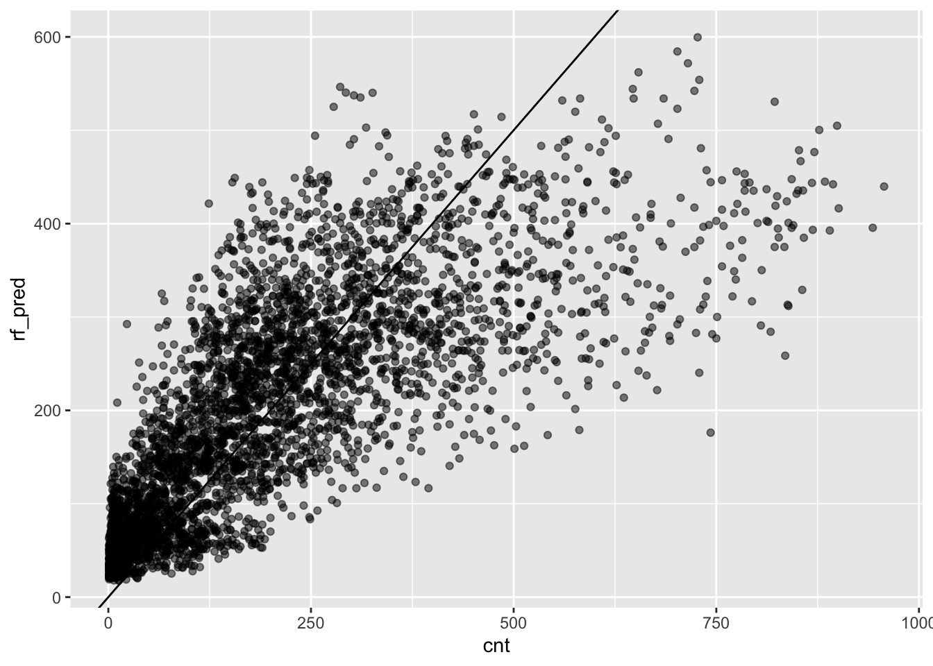
This looks better than what we got with linear regression, but there is
still room for improvement. The issue of large errors for large values of
cnt is still present despite being less severe.
Cross Validation
Obviously we are not limited to a simple workflow of fitting models and predicting afterwards. Given that we are appearing to overfit with our random forest model, cross validation is an option we should explore, so we get a reasonable estimate of which metrics we can expect.
Cross validation in tidymodels is also a very simple process. The functions
used here are part of the rsample and tune packages from the tidymodels
family.
First we create our folds, ten in this case.
training_cv <- vfold_cv(training, v = 10)This does create a list of splits similar to what we created with
initial_split above.
Carrying out the fitting and predicting on this list is equally simple.
rf_cv <- fit_resamples(
  formula = cnt ~ .,
  model = rf,
  resamples = training_cv
)
The formula is the usual definition of dependent variable and predictors,
the model is our model specified above and the resamples are the
folds we just created.
And we can have a look at the metrics generated here.
rf_cv %>% collect_metrics()## # A tibble: 2 x 5
## .metric .estimator mean n std_err
## <chr> <chr> <dbl> <int> <dbl>
## 1 rmse standard 115. 10 0.700
## 2 rsq standard 0.607 10 0.00525We can also get the range of RMSE values doing a bit of wrangling with the results.
rf_cv %>%
  unnest(.metrics) %>%
  filter(.metric == "rmse") %>%
  select(.estimate) %>%
  deframe() %>%
  range()
## [1] 111.9653 119.9293The values we got here are a better estimate on how the model would perform on previously unseen data and this is comparable to what we have seen on our test data.
Model tuning
With many kinds of models we have the option to tune hyperparameters, this
is where the tools provided by the tune package come in.
Hyperparameter tuning is often not an exact science but boils down to carrying
out a grid search, i.e. trying a pre-defined range of values for a set of
hyperparameters and see how the model performs.
Most likely you want to tune more than one parameter, but for demonstration
purposes we will just tune the mtry parameter for rand_forest,
controlling the amount of predictors to sample at each tree split.
rf_grid <- rand_forest(mtry = tune()) %>%
  set_mode("regression") %>%
  set_engine("ranger")
We can then conduct the grid search. Be aware that doing this might take
quite some time, depending on the model complexity and the amount of data.
You can set the control parameter verbose to TRUE to get updates about
the status.
rf_grid_fit <- tune_grid(
  formula = cnt ~ .,
  model = rf_grid,
  resamples = training_cv,
  control = control_grid(verbose = FALSE)
)
You can then extract the best parameters from the fitted grid. Make sure to specify whether you want to maximize the metric of interest, with RMSE you obviously want the lowest value.
rf_grid_fit %>% show_best(metric = "rmse", maximize = FALSE)## # A tibble: 5 x 6
## mtry .metric .estimator mean n std_err
## <int> <chr> <chr> <dbl> <int> <dbl>
## 1 9 rmse standard 112. 10 0.858
## 2 12 rmse standard 112. 10 0.873
## 3 13 rmse standard 112. 10 0.874
## 4 15 rmse standard 112. 10 0.841
## 5 18 rmse standard 113. 10 0.805Apparently an mtry value of 9 provides the lowest error, but comparing
it to the other values here we are clearly in the range of diminishing returns
for the given circumstances.
Conclusions
The tidymodels family of packages sure looks promising.
This post has only shown the tip of the iceberg regarding what you can do,
however this is hopefully good enough to get you up to speed.
As of now you probably want to be careful putting tidymodels to productive use
as those packages have not matured yet and things are likely changing quite
significantly in the future, so stuff might break when updating packages.
Additionally one thing that has not made it into tidymodels yet is mixed
modelling, which is something that might be essential for you.
There is the option to add your own model interfaces, but I have not given this
a try yet and thus am unsure whether this is suitable for mixed models.
To sum things up: tidymodels is likely here to stay and you might want to
familiarise yourself with it, but do not fully rely on it yet.