Statistics, Science, Random Ramblings
A blog about data and other interesting things
Basic maps in R with ggplot2
This is a guide to simple choropleth maps in R using ggplot2 and geom_sf().
The ability to plot map data represented as simple features was introduced
to ggplot2 not that long ago, such data can be easily accessed using the
rnaturalearth package.
First of all, as I just learned this recently as well: choropleth maps are maps in which data is represented by shading areas according to some value. At the end of this post we will have a map showing the population density of the states (first administrative subdivision) of Finland by hue, which is pretty much a textbook example of a choropleth map.
Getting Map Data in R
Large amounts of good-quality map data can be obtained by using the
rnaturalearth package. Specifying returnclass = sf option in function calls
you can get simple features data which is easy to work with and is what
geom_sf expects.
library("rnaturalearth")
mapData <- ne_countries(scale = 10, continent = c("Europe"), returnclass = "sf")
Note that you can set the scale option to a different value (50 or 110) to get
a lower resolution map, which leads to much faster plotting at the cost of a
map that does not look as nice..
Let’s have a look at what we have:
library("tidyverse")
glimpse(mapData)
## Observations: 51
## Variables: 95
## $ featurecla <chr> "Admin-0 country", "Admin-0 country", "Admin-0 countr…
## $ scalerank <int> 0, 0, 0, 0, 0, 0, 0, 0, 0, 0, 0, 0, 0, 0, 0, 0, 0, 0,…
## $ labelrank <int> 2, 3, 4, 5, 2, 5, 2, 6, 5, 3, 3, 3, 6, 2, 6, 6, 6, 2,…
## $ sovereignt <chr> "France", "Ukraine", "Belarus", "Lithuania", "Russia"…
## $ sov_a3 <chr> "FR1", "UKR", "BLR", "LTU", "RUS", "CZE", "DEU", "EST…
## $ adm0_dif <int> 1, 0, 0, 0, 0, 0, 0, 0, 0, 0, 0, 1, 0, 0, 0, 0, 0, 0,…
## $ level <int> 2, 2, 2, 2, 2, 2, 2, 2, 2, 2, 2, 2, 2, 2, 2, 2, 2, 2,…
## $ type <chr> "Country", "Sovereign country", "Sovereign country", …
## $ admin <chr> "France", "Ukraine", "Belarus", "Lithuania", "Russia"…
## $ adm0_a3 <chr> "FRA", "UKR", "BLR", "LTU", "RUS", "CZE", "DEU", "EST…
## $ geou_dif <int> 0, 0, 0, 0, 0, 0, 0, 0, 0, 0, 0, 0, 0, 0, 0, 0, 0, 0,…
## $ geounit <chr> "France", "Ukraine", "Belarus", "Lithuania", "Russia"…
## $ gu_a3 <chr> "FRA", "UKR", "BLR", "LTU", "RUS", "CZE", "DEU", "EST…
## $ su_dif <int> 0, 0, 0, 0, 0, 0, 0, 0, 0, 0, 0, 0, 0, 0, 0, 0, 0, 0,…
## $ subunit <chr> "France", "Ukraine", "Belarus", "Lithuania", "Russia"…
## $ su_a3 <chr> "FRA", "UKR", "BLR", "LTU", "RUS", "CZE", "DEU", "EST…
## $ brk_diff <int> 0, 0, 0, 0, 0, 0, 0, 0, 0, 0, 0, 0, 0, 0, 0, 0, 0, 0,…
## $ name <chr> "France", "Ukraine", "Belarus", "Lithuania", "Russia"…
## $ name_long <chr> "France", "Ukraine", "Belarus", "Lithuania", "Russian…
## $ brk_a3 <chr> "FRA", "UKR", "BLR", "LTU", "RUS", "CZE", "DEU", "EST…
## $ brk_name <chr> "France", "Ukraine", "Belarus", "Lithuania", "Russia"…
## $ brk_group <chr> NA, NA, NA, NA, NA, NA, NA, NA, NA, NA, NA, NA, NA, N…
## $ abbrev <chr> "Fr.", "Ukr.", "Bela.", "Lith.", "Rus.", "Cz.", "Ger.…
## $ postal <chr> "F", "UA", "BY", "LT", "RUS", "CZ", "D", "EST", "LV",…
## $ formal_en <chr> "French Republic", "Ukraine", "Republic of Belarus", …
## $ formal_fr <chr> NA, NA, NA, NA, NA, "la République tchèque", NA, NA, …
## $ name_ciawf <chr> "France", "Ukraine", "Belarus", "Lithuania", "Russia"…
## $ note_adm0 <chr> NA, NA, NA, NA, NA, NA, NA, NA, NA, NA, NA, NA, NA, N…
## $ note_brk <chr> NA, NA, NA, NA, NA, NA, NA, NA, NA, NA, NA, NA, NA, N…
## $ name_sort <chr> "France", "Ukraine", "Belarus", "Lithuania", "Russian…
## $ name_alt <chr> NA, NA, NA, NA, NA, "Cesko", NA, NA, NA, NA, NA, NA, …
## $ mapcolor7 <int> 7, 5, 1, 6, 2, 1, 2, 3, 4, 5, 1, 4, 1, 3, 5, 1, 2, 4,…
## $ mapcolor8 <int> 5, 1, 1, 3, 5, 1, 5, 2, 7, 3, 4, 1, 7, 2, 3, 4, 2, 5,…
## $ mapcolor9 <int> 9, 6, 5, 3, 7, 2, 5, 1, 6, 8, 2, 4, 3, 1, 7, 1, 3, 5,…
## $ mapcolor13 <int> 11, 3, 11, 9, 7, 6, 1, 10, 13, 12, 4, 6, 7, 8, 3, 6, …
## $ pop_est <chr> "67106161", "44033874", "9549747", "2823859", "142257…
## $ pop_rank <int> 16, 15, 13, 12, 17, 14, 16, 12, 12, 13, 13, 13, 11, 1…
## $ gdp_md_est <dbl> 2699000, 352600, 165400, 85620, 3745000, 350900, 3979…
## $ pop_year <int> 2017, 2017, 2017, 2017, 2017, 2017, 2017, 2017, 2017,…
## $ lastcensus <int> NA, 2001, 2009, 2011, 2010, 2011, 2011, 2000, 2011, 2…
## $ gdp_year <int> 2016, 2016, 2016, 2016, 2016, 2016, 2016, 2016, 2016,…
## $ economy <chr> "1. Developed region: G7", "6. Developing region", "6…
## $ income_grp <chr> "1. High income: OECD", "4. Lower middle income", "3.…
## $ wikipedia <int> NA, NA, NA, NA, NA, NA, NA, NA, NA, NA, NA, NA, NA, N…
## $ fips_10_ <chr> "FR", "UP", "BO", "LH", "RS", "EZ", "GM", "EN", "LG",…
## $ iso_a2 <chr> NA, "UA", "BY", "LT", "RU", "CZ", "DE", "EE", "LV", N…
## $ iso_a3 <chr> NA, "UKR", "BLR", "LTU", "RUS", "CZE", "DEU", "EST", …
## $ iso_a3_eh <chr> "FRA", "UKR", "BLR", "LTU", "RUS", "CZE", "DEU", "EST…
## $ iso_n3 <chr> "250", "804", "112", "440", "643", "203", "276", "233…
## $ un_a3 <chr> "250", "804", "112", "440", "643", "203", "276", "233…
## $ wb_a2 <chr> "FR", "UA", "BY", "LT", "RU", "CZ", "DE", "EE", "LV",…
## $ wb_a3 <chr> "FRA", "UKR", "BLR", "LTU", "RUS", "CZE", "DEU", "EST…
## $ woe_id <int> -90, 23424976, 23424765, 23424875, 23424936, 23424810…
## $ woe_id_eh <int> 23424819, 23424976, 23424765, 23424875, 23424936, 234…
## $ woe_note <chr> "Includes only Metropolitan France (including Corsica…
## $ adm0_a3_is <chr> "FRA", "UKR", "BLR", "LTU", "RUS", "CZE", "DEU", "EST…
## $ adm0_a3_us <chr> "FRA", "UKR", "BLR", "LTU", "RUS", "CZE", "DEU", "EST…
## $ adm0_a3_un <int> NA, NA, NA, NA, NA, NA, NA, NA, NA, NA, NA, NA, NA, N…
## $ adm0_a3_wb <int> NA, NA, NA, NA, NA, NA, NA, NA, NA, NA, NA, NA, NA, N…
## $ continent <chr> "Europe", "Europe", "Europe", "Europe", "Europe", "Eu…
## $ region_un <chr> "Europe", "Europe", "Europe", "Europe", "Europe", "Eu…
## $ subregion <chr> "Western Europe", "Eastern Europe", "Eastern Europe",…
## $ region_wb <chr> "Europe & Central Asia", "Europe & Central Asia", "Eu…
## $ name_len <int> 6, 7, 7, 9, 6, 7, 7, 7, 6, 6, 6, 7, 10, 7, 9, 7, 6, 5…
## $ long_len <int> 6, 7, 7, 9, 18, 14, 7, 7, 6, 6, 6, 7, 10, 7, 9, 7, 6,…
## $ abbrev_len <int> 3, 4, 5, 5, 4, 3, 4, 4, 4, 4, 4, 4, 4, 5, 4, 4, 4, 3,…
## $ tiny <int> NA, NA, NA, NA, NA, NA, NA, NA, NA, NA, NA, NA, 5, NA…
## $ homepart <int> 1, 1, 1, 1, 1, 1, 1, 1, 1, 1, 1, 1, 1, 1, 1, 1, 1, 1,…
## $ min_zoom <dbl> 0, 0, 0, 0, 0, 0, 0, 0, 0, 0, 0, 0, 0, 0, 0, 0, 0, 0,…
## $ min_label <dbl> 1.7, 3.0, 3.0, 4.0, 1.7, 4.0, 1.7, 3.0, 4.0, 3.0, 3.0…
## $ max_label <dbl> 6.7, 7.0, 8.0, 9.0, 5.2, 9.0, 6.7, 8.0, 9.0, 7.0, 7.0…
## $ ne_id <chr> "1159320637", "1159321345", "1159320427", "1159321029…
## $ wikidataid <chr> "Q142", "Q212", "Q184", "Q37", "Q159", "Q213", "Q183"…
## $ name_ar <chr> NA, NA, NA, NA, NA, NA, NA, NA, NA, NA, NA, NA, NA, N…
## $ name_bn <chr> NA, NA, NA, NA, NA, NA, NA, NA, NA, NA, NA, NA, NA, N…
## $ name_de <chr> "Frankreich", "Ukraine", "Weißrussland", "Litauen", "…
## $ name_en <chr> "France", "Ukraine", "Belarus", "Lithuania", "Russia"…
## $ name_es <chr> "Francia", "Ucrania", "Bielorrusia", "Lituania", "Rus…
## $ name_fr <chr> "France", "Ukraine", "Biélorussie", "Lituanie", "Russ…
## $ name_el <chr> NA, NA, NA, NA, NA, NA, NA, NA, NA, NA, NA, NA, NA, N…
## $ name_hi <chr> NA, NA, NA, NA, NA, NA, NA, NA, NA, NA, NA, NA, NA, N…
## $ name_hu <chr> "Franciaország", "Ukrajna", "Fehéroroszország", "Litv…
## $ name_id <chr> "Perancis", "Ukraina", "Belarus", "Lituania", "Rusia"…
## $ name_it <chr> "Francia", "Ucraina", "Bielorussia", "Lituania", "Rus…
## $ name_ja <chr> NA, NA, NA, NA, NA, NA, NA, NA, NA, NA, NA, NA, NA, N…
## $ name_ko <chr> NA, NA, NA, NA, NA, NA, NA, NA, NA, NA, NA, NA, NA, N…
## $ name_nl <chr> "Frankrijk", "Oekraïne", "Wit-Rusland", "Litouwen", "…
## $ name_pl <chr> "Francja", "Ukraina", "Bialorus", "Litwa", "Rosja", "…
## $ name_pt <chr> "França", "Ucrânia", "Bielorrússia", "Lituânia", "Rús…
## $ name_ru <chr> NA, NA, NA, NA, NA, NA, NA, NA, NA, NA, NA, NA, NA, N…
## $ name_sv <chr> "Frankrike", "Ukraina", "Vitryssland", "Litauen", "Ry…
## $ name_tr <chr> "Fransa", "Ukrayna", "Beyaz Rusya", "Litvanya", "Rusy…
## $ name_vi <chr> "Pháp", "Ukraina", "Belarus", "Litva", "Nga", NA, NA,…
## $ name_zh <chr> NA, NA, NA, NA, NA, NA, NA, NA, NA, NA, NA, NA, NA, N…
## $ geometry <MULTIPOLYGON [°]> MULTIPOLYGON (((-54.11153 2..., MULTIPOL…That is a lot of data. In theory we do not need much of it, just for plotting the geometry column should be enough. So let’s reduce the data:
mapData <- select(mapData, name, geometry)Making Maps
It is straightforward to plot this (but takes a moment):
ggplot(mapData) + geom_sf()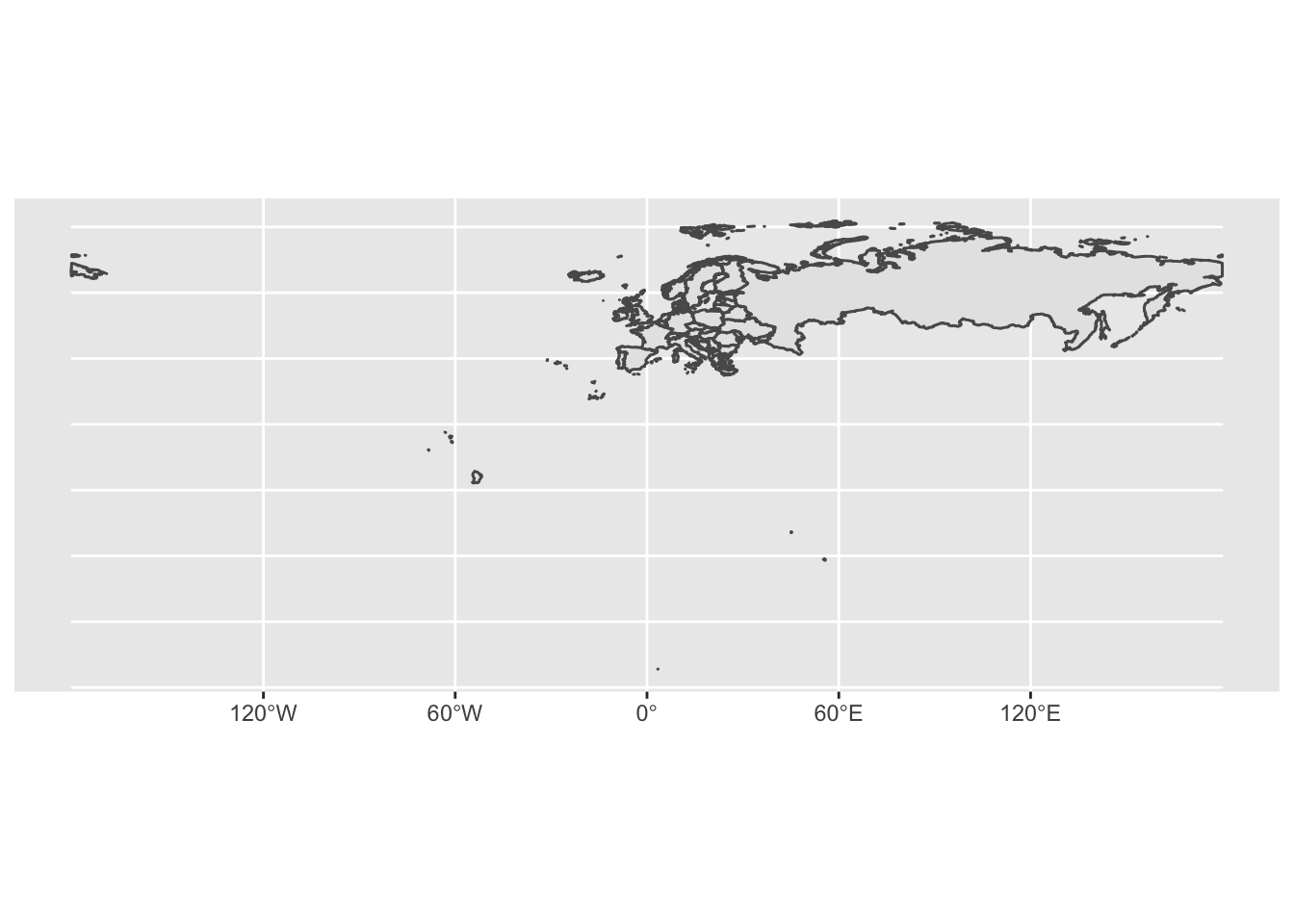
That might not exactly be what you expected, but we can work with this. It is not difficult to limit the map to a specific area, colour stuff, etc.
When we have an idea of the area we want to plot, it is easy to limit the map:
ggplot(data = mapData) +
    geom_sf(color = "black", fill = "antiquewhite") +
    coord_sf(xlim = c(18, 32), ylim = c(58, 71)) +
    labs(title = "Finland") +
    theme(panel.background = element_rect(fill = "aliceblue"))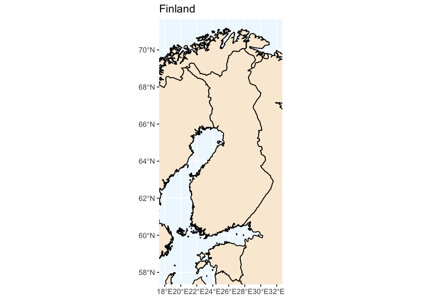
This does already look very map-ish.
The xlim and ylim arguments to coord_sf limit the map to the specified
coordinate ranges, adding some colour makes the map-look complete.
Fine-Tuning The Map
Now let’s do something useful with it.
First, get the states of Finland (first administrative subdivision, maakunta in Finnish).
fi_states <- ne_states(country = "finland", returnclass = "sf")
fi_states <- select(fi_states, name, geometry)
glimpse(fi_states)
## Observations: 18
## Variables: 2
## $ name <chr> "Lapland", "Northern Ostrobothnia", "Kainuu", "North Ka…
## $ geometry <MULTIPOLYGON [°]> MULTIPOLYGON (((27.86691 70..., MULTIPOLYG…ggplot() +
geom_sf(data = mapData, colour = "grey50", fill = "antiquewhite") +
geom_sf(data = fi_states, aes(fill = name),
colour = "black", alpha = .5) +
guides(fill = FALSE) +
coord_sf(xlim = c(18, 32), ylim = c(58, 71)) +
labs(title = "Finland") +
theme(panel.background = element_rect(fill = "aliceblue"))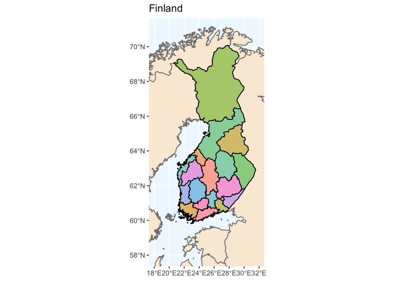
Note that there are two calls to geom_sf here. The first contains the
background map data specifying its appearance, the second one is for the data
that we want to visualise containing a call to aes. We include the line
guides(fill = FALSE) to avoid having a legend appear in the map. Depending on
what you want to accomplish having a legend might be useful, though.
This data is missing Åland, which is much more autonomous than the other regions,
but nonetheless part of Finland. The data for Åland is contained in a different
row in the map data for Europe and it can be added to fi_states easily using
rbind:
aland <- filter(mapData, name == "Åland")
fi_states <- rbind(fi_states, aland)
ggplot() +
    geom_sf(data = mapData, colour = "grey50", fill = "antiquewhite") +
    geom_sf(data = fi_states, aes(fill = name),
            colour = "black", alpha = .5) +
    guides(fill = FALSE) +
    coord_sf(xlim = c(18, 32), ylim = c(58, 71)) +
    labs(title = "Finland") +
    theme(panel.background = element_rect(fill = "aliceblue"))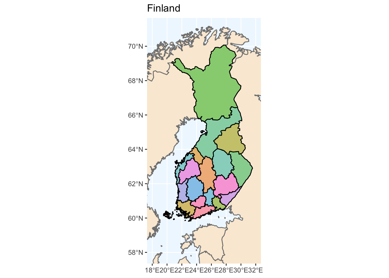
The map now looks like we have successfully included the previously missing Åland.
Adding Data
We can add some information about the population of the regions of Finland. The data is available from Statistics Finland’s 2018 Finland in Figures report.
The region names were modified to match those in the date from the
rnaturalearth package.
maakunta <- tribble(
                    ~Region, ~Population.density, ~Population, ~Annual.change, ~Share.of.total.population, ~Excess.of.births,
                  "Uusimaa",                 182,     1655624,            1.1,                         30,               2.7,
           "Finland Proper",                  45,      477677,            0.4,                        8.7,              -1.6,
                "Satakunta",                  28,      220398,           -0.6,                          4,              -4.5,
          "Tavastia Proper",                  33,      172720,           -0.6,                        3.1,              -2.2,
                "Pirkanmaa",                  41,      512081,            0.5,                        9.3,              -0.2,
              "Päijät-Häme",                  39,      201228,           -0.2,                        3.6,              -3.2,
              "Kymenlaakso",                  34,      175511,           -1.2,                        3.2,              -5.8,
            "South Karelia",                  24,      129865,           -0.5,                        2.4,              -5.2,
         "Southern Savonia",                  10,      147194,           -1.2,                        2.7,              -7.7,
         "Northern Savonia",                  15,      246653,           -0.5,                        4.5,              -3.5,
            "North Karelia",                   9,      162986,           -0.7,                          3,              -4.6,
          "Central Finland",                  17,      276031,           -0.1,                          5,              -1.7,
    "Southern Ostrobothnia",                  14,      190910,           -0.5,                        3.5,              -1.7,
             "Ostrobothnia",                  23,      180945,           -0.3,                        3.3,              -0.1,
     "Central Ostrobothnia",                  14,       68780,           -0.4,                        1.2,               1.2,
    "Northern Ostrobothnia",                  11,      411856,            0.2,                        7.5,               2.8,
                   "Kainuu",                   4,       73959,           -1.1,                        1.3,              -6.1,
                  "Lapland",                   2,      179223,           -0.5,                        3.3,              -3.5,
                    "Åland",                  19,       29489,            0.9,                        0.5,               1.5)
This can easily be merged into the map data using left_join from dplyr:
fi_states <- left_join(fi_states, maakunta, by = c("name" = "Region"))The information available in the maakunta dataset can now be plotted as well
(you might want to examine the merged data set beforehand).
myBreaks <- 2 ^ c(0:4) * 10
ggplot() +
geom_sf(data = mapData, colour = "grey50", fill = "antiquewhite") +
geom_sf(data = fi_states, aes(fill = Population.density), colour = "black",
) +
scale_fill_gradient(low = "lavenderblush", high = "deeppink4",
trans = "log", breaks = myBreaks) +
coord_sf(xlim = c(18, 32), ylim = c(58, 71), datum = NA) +
labs(title = "Population Density of Finland",
fill = "Inhabitants\nper km²",
x = "Latitude", y = "Longitude") +
theme_void() +
theme(panel.background = element_rect(fill = "aliceblue"))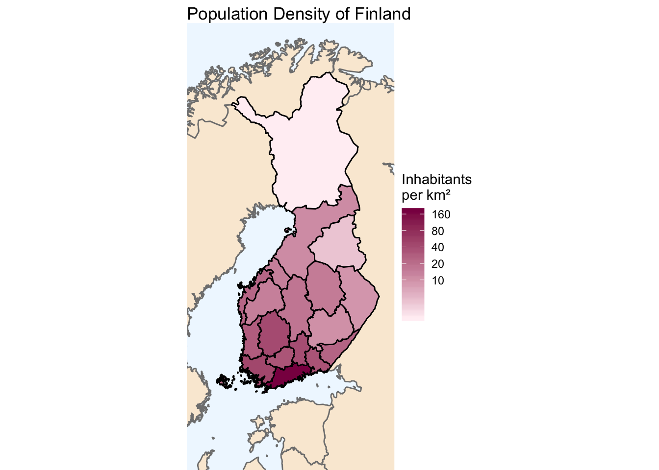 Before plotting we create a vector
 myBreaks that contains custom tick marks
for our log scale. A log scale for population density makes sense here as span of
the values is rather big and differences for most regions would become
indistinguishable.
Further cosmetic tweaks in this map are the datum = NA option in coord_sf()
to hide the grid lines and the call to theme_void() that essentially hides all
other unwanted elements of the map.
We can see from the map, that perhaps unsurprisingly, the population density of Finland is much lower in the north than in the south with the density being highest in the area of Helsinki (state of Uusima).
Finally, we can save the map to disk:
ggplot2::ggsave("finland_population_density.png",
                width = 6, height = 12, dpi = 300)
Concluding Remarks
We have seen that creating informative maps in R is not hard. However there are a few things worth noting:
- Finding accurate map data for specific regions can be hard. If you are lucky there is an open data site for what you are interested in, if not things become much more tricky.
- Maps are sometimes not as simple as it seems, for example when dealing with disputed borders.
- While simple features data was used here, there are many more ways to store and use geo-data in R.