library("dustrees")
library("dplyr")
library("ggplot2")
library("tidyr")
data("trees")
data("dus_city")
data("dus_quarters")

glimpse(trees)

## Rows: 2,190
## Columns: 9
## $ lat        <dbl> 51.22519, 51.22525, 51.21988, 51.21558, 51.22635, 51.21815…
## $ lon        <dbl> 6.772675, 6.790152, 6.778963, 6.770085, 6.786974, 6.789049…
## $ reason     <chr> "abgestorben", NA, NA, NA, NA, NA, NA, NA, "nur noch Stamm…
## $ id         <chr> "1032", "1591", "2190", "2326", "2412", "2559", "2661", "2…
## $ species_de <chr> "scheinakazie", "scheinakazie", "kastanie", "platane", "sc…
## $ street     <chr> "Flinger Straße", "Hohenzollernstraße", "Königsallee", "Ko…
## $ circ       <dbl> NA, NA, NA, NA, NA, NA, NA, NA, 380, 280, 340, 240, 350, 1…
## $ year       <dbl> 2018, 2018, 2018, 2018, 2018, 2018, 2018, 2018, 2018, 2018…
## $ part       <dbl> 1, 1, 1, 1, 1, 1, 1, 1, 1, 1, 1, 1, 1, 1, 1, 1, 1, 1, 1, 1…

Mapping cut-down trees

Let’s begin by mapping where trees were cut-down in the city.

source_str <- "Data Source: Open Data Düsseldorf"

ggplot(trees) +
    geom_sf(data = dus_city, fill = "white") +
    geom_point(aes(x = lon, y = lat), size = 0.75, alpha = .5, 
               colour = "green4") +
    facet_grid(rows = .~paste(year, part)) +
    labs(x = "", y = "", title = "Positions of cut-down trees over time",
         subtitle = "in Düsseldorf/Germany during 2018/19",
         caption = source_str) +
    coord_sf(datum = NA) +
    theme_minimal()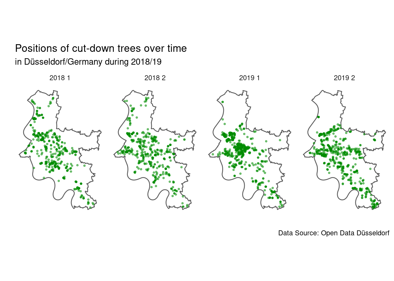

It looks like the most trees are cut down in a central area of the city, while especially in the north and north-east of the city only a few trees were cut down. This might suggest that the busier part of the city has more detrimental conditions for trees and/or there are more trees in that area. Just from the plot alone this would be a pretty bold conclusion though.

As a next step we can have a look at trees that were cut-down by quarter

in_quarter <- apply(trees, 1, function(x) {
  find_containing_geo(dus_quarters, "Description", c(x["lon"], x["lat"]) %>% 
                        as.numeric())
}) 
trees$quarter <- unlist(in_quarter)

Now we can count the amount of cut down trees in the quarters.

cut_down_quarter <- trees %>% 
  group_by(year, part, .drop = FALSE) %>% 
  count(quarter, name = "cnt") %>% 
  ungroup() %>% 
  complete(quarter, year, part)

cut_down_quarter_sf <- cut_down_quarter %>% 
  left_join(dus_quarters, ., by = c("Description" = "quarter"))

And we are ready to plot.

ggplot(cut_down_quarter_sf) +
  aes(fill = cnt) +
  geom_sf() +
  facet_grid(rows = .~paste(year, part)) +
  labs(x = "", y = "", fill = "Cut-Down Trees",
       title = "Amount of cut-down trees over time",
       subtitle = "in quarters of Düsseldorf during 2018/19",
       caption = source_str) +
  scale_fill_continuous(low = "antiquewhite", high = "red4", 
                        na.value = "grey90") +
  coord_sf(datum = NA) +
  theme_minimal() +
  theme(legend.position = "bottom")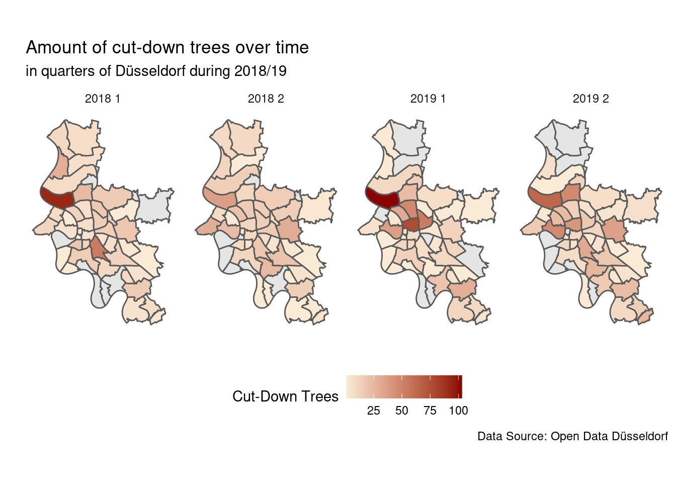

There is one quarter that is clearly standing out a bit north of the city centre.

cut_down_quarter %>% 
  slice_max(cnt, n = 10)

## # A tibble: 10 x 4
##    quarter     year  part   cnt
##    <chr>      <dbl> <dbl> <int>
##  1 Stockum     2019     1   103
##  2 Stockum     2018     1    93
##  3 Pempelfort  2019     1    77
##  4 Stockum     2019     2    64
##  5 Düsseltal   2019     1    54
##  6 Oberbilk    2018     1    54
##  7 Derendorf   2019     1    47
##  8 Oberkassel  2019     2    47
##  9 Unterrath   2019     2    47
## 10 Pempelfort  2019     2    41

That quarter is Stockum. A quick web search reveals that apparently numerous trees in that are were cut down for constructions on a sound-barrier along an autobahn. Furthermore there were apparently issues with fungus infections in the area.

For the data we have we can look whether Stockum is the area the heaviest affected by cutting-down of trees in the city of Düsseldorf.

quarter_total <- trees %>% 
  count(quarter, name = "cnt") %>% 
  drop_na(quarter)

max_quarters <- quarter_total %>% slice_max(cnt, n = 5)
max_quarters

## # A tibble: 5 x 2
##   quarter      cnt
##   <chr>      <int>
## 1 Stockum      297
## 2 Pempelfort   136
## 3 Oberkassel   112
## 4 Oberbilk     110
## 5 Unterrath    104

Apparently this is indeed the case.

We can also check which are the least affected quarters.

min_quarters <- quarter_total %>% slice_min(cnt, n = 5)
min_quarters

## # A tibble: 5 x 2
##   quarter     cnt
##   <chr>     <int>
## 1 Flehe         1
## 2 Hafen         1
## 3 Itter         1
## 4 Knittkuhl     1
## 5 Hamm          2

Let’s visualise them.

minmax_map <- dus_quarters %>% 
  mutate(minmax = case_when(
    .$Description %in% max_quarters$quarter ~ "most",
    .$Description %in% min_quarters$quarter ~ "least",
    TRUE ~ NA_character_
  ))

ggplot(minmax_map) +
  aes(fill = minmax) +
  geom_sf() +
  scale_fill_viridis_d(na.translate = FALSE) +
  labs(x = "", y = "", fill = "",
       title = "Most/least cut-down trees",
       subtitle = "in quarters of Düsseldorf during 2018/19",
       caption = source_str) +
  coord_sf(datum = NA) +
  theme_minimal() +
  theme(legend.position = "bottom")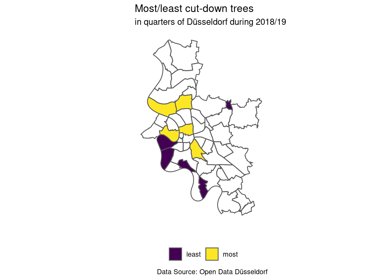

We can see that four of the quarters with only few cut-down trees are near the Rhine (the squiggly left border of the city).

Reasons for cutting-down trees

As we have now looked at where trees where cut-down in Düsseldorf, now let’s examine why they where cut down.

Our data does contain a column on the reason, but it can not be used as is due to the variety of reasons given and the varying amount of detail.

Let’s have a quick look first:

head(unique(trees$reason), n = 10)

##  [1] "abgestorben"                    NA                              
##  [3] "nur noch Stamm"                 "Morschungen im Stammfußbereich"
##  [5] "Sturmschaden"                   "Pilzbefall (Lackporling) "     
##  [7] "Morschungen am Kronenansatz"    "Morschungen am Stammfuß"       
##  [9] "Pilzbefall (Schwefelporling)"   "Komplexerkrankung"

Obviously the reasons are in German. A good strategy here is probably to match certain keywords to the column and one-hot encode the reasons. We do this for 10 common reasons in the data.

trees <- trees %>% 
  mutate(reason = tolower(reason)) %>% 
  mutate(reason_fungus = ifelse(grepl("pilz", .$reason), 1, 0),
         reason_storm = ifelse(grepl("sturm", .$reason), 1, 0),
         reason_rot = ifelse(grepl("f(ae|ä|a)ul|morsch", .$reason), 1, 0),
         reason_dead = ifelse(grepl("gestorben|sterbend", .$reason), 1, 0),
         reason_vandalism = ifelse(
           grepl("sachbeschädigung|vandalismus", .$reason), 1, 0),
         reason_tear = ifelse(grepl("riss", .$reason), 1, 0),
         reason_dry = ifelse(grepl("trocken", .$reason), 1, 0),
         reason_trunkdamage = ifelse(grepl("stammsch(ä|a)den", .$reason), 1, 0),
         reason_construction = ifelse(grepl("baumaßnahme", .$reason), 1, 0),
         reason_slant = ifelse(grepl("schrägstand", .$reason), 1, 0)) %>% 
  mutate(reason_other_or_none = ifelse(
    rowSums(trees[grepl("reason_", colnames(trees))]) == 0, 1, 0))

We can now verify that this covers most of the data, by looking at the amount of trees where no reason is coded in the newly added columns.

other_reasons <- trees %>% 
  filter(rowSums(trees[grepl("reason_", colnames(trees))]) == 0 & 
         !is.na(reason)) %>% 
  select(reason) %>% 
  tibble::deframe() %>% 
  unique() %>% 
  length()
other_reasons

## [1] 0

Compare this with the total amount of non-NA reasons:

no_reason <- trees %>% 
  filter(!is.na(reason)) %>% 
  nrow()
no_reason

## [1] 2092

Both of these groups are merged into the reason other_or_none column. Let’s map the reasons and see whether there are patterns.

reasons <- reasons_long_data(trees, id, lat, lon, quarter)

Now that we have long data the plot is easily done.

reasons %>% 
  mutate(reason = gsub("_or_", "/", .$reason)) %>% 
  ggplot() + 
  geom_sf(data = dus_city, fill = "white") + 
  geom_point(aes(x = lon, y = lat, colour = reason), alpha = .3) +
  scale_colour_viridis_d(na.translate = FALSE) +
  facet_wrap(.~reason, nrow = 2) + 
  coord_sf(datum = NA) + 
  labs(x = "", y = "", title = "Reasons for cutting down of trees",
       subtitle = "in the city of Düsseldorf during 2018/19",
       caption = source_str) +
  theme_minimal() + 
  guides(colour = FALSE)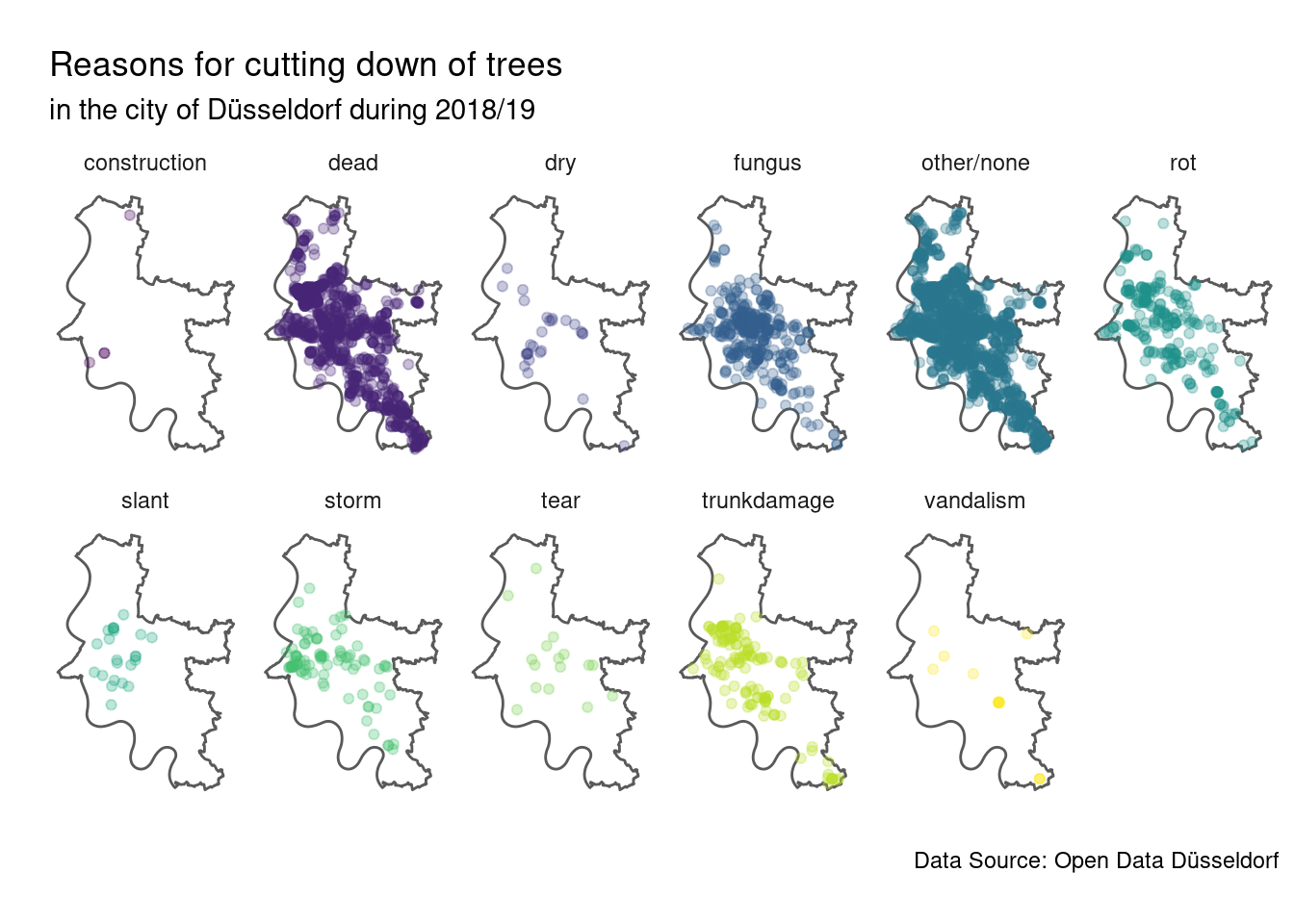

It does not seem like there are obvious patterns, but once a reason is common enough it is more or less present all over the city. The most common reasons for cutting-down trees in the city of Düsseldorf appear to be that the trees were dead, infected by fungi or rotting. Note however that it is not unlikely that there is some overlap between those reasons, as at the end of the day the reason for cutting-down is given from a free text field in the data. Also we should keep in mind that for many cut-down trees no reasons was given why they were cut down.

Let’s investigate a bit more.

reasons %>%
  count(reason, name = "prop") %>% 
  mutate(prop = round(prop / sum(prop), 3)) %>% 
  arrange(desc(prop)) 

## # A tibble: 11 x 2
##    reason         prop
##    <chr>         <dbl>
##  1 other_or_none 0.516
##  2 dead          0.256
##  3 fungus        0.097
##  4 rot           0.058
##  5 trunkdamage   0.033
##  6 storm         0.02 
##  7 dry           0.006
##  8 slant         0.005
##  9 tear          0.004
## 10 vandalism     0.004
## 11 construction  0.001

For about half of the data no reason for cutting down was specified, while about a quarter of the trees in the dataset had to be cut down because they were dead.

What happened in Stockum?

In the mapping part we have seen that in the quarter of Stockum by far the most trees have been cut down. We should have a closer look at why they were cut down, maybe some patterns emerge.

So first filter for the quarter of Stockum.

stockum <- trees %>% filter(quarter == "Stockum")

Then extract the reasons.

stockum_reasons <- reasons_long_data(stockum, id, lat, lon)

And get the proportions of reasons.

reasons_prop <- stockum_reasons %>% 
  count(reason, name = "prop") %>% 
  mutate(prop = round(prop / sum(prop), 3)) %>% 
  arrange(desc(prop))

reasons_prop

## # A tibble: 9 x 2
##   reason         prop
##   <chr>         <dbl>
## 1 other_or_none 0.523
## 2 dead          0.315
## 3 rot           0.065
## 4 trunkdamage   0.053
## 5 storm         0.018
## 6 fungus        0.016
## 7 slant         0.005
## 8 dry           0.004
## 9 vandalism     0.002

Let’s also map the trees and the most common reasons.

stockum_sf <- dus_quarters %>% filter(Description == "Stockum")

stockum_reasons %>% 
  filter(reason %in% reasons_prop$reason[1:4]) %>% 
  ggplot() +
    geom_sf(data = stockum_sf, fill = "white") +
    geom_point(aes(x = lon, y = lat, colour = reason), alpha = .8) +
    scale_color_viridis_d(na.translate = FALSE) +
    coord_sf(datum = NA) +
    theme_minimal() +
    guides(colour = FALSE) +
    labs(x = "", y = "", 
         title = "Cut-down trees in the quarter of Stockum, Düsseldorf",
         subtitle = "With reasons for cutting-down in 2018/19",
         caption = source_str, colour = "Reason") +
    facet_wrap(.~reason, ncol = 2, nrow = 2)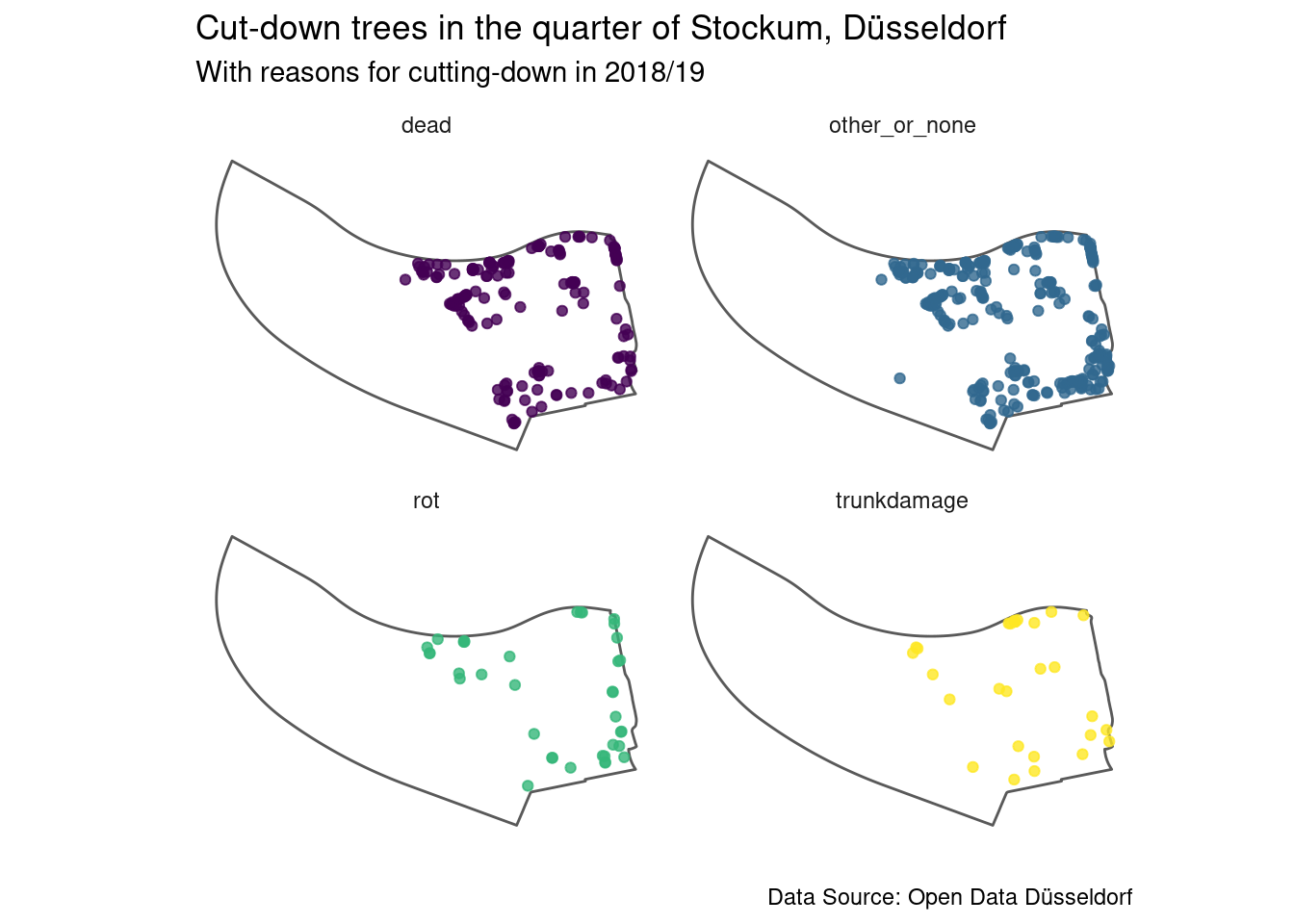

Now we should have closer look at what Stockum looks like on a map (yes, we could use leaflet but this requires connecting to external sites). The Northern border of Stockum is the A44 autobahn, the Eastern border is the B8 main road, in the south it is a park (Nordpark) and in the West it is the Rhine. Interestingly, a very green part of the quarter at the Rhine does not contain locations of cut-down trees. Examining the map it becomes apparent that the cut-down trees are essentially along the roads forming the border of the quarter, in the area of the trade fair and some in the park. The reason for cutting-down most of the trees here is that they were dead, which makes me wonder if being next to a busy street is not exactly healthy for trees (I am not an expert on trees, though). However the amount of trees that were cut-down for which no reason was given is larger and exhibits the same pattern. Those trees might have been cut-down for traffic-safety or construction reasons, but this data set alone does not contain any more in-depth information.

Species of trees

Finally, let’s also have a quick look at patterns that might emerge for the most common types of trees.

There is quite a large amount of unique types of trees in the data.

length(unique(trees$species_de))

## [1] 158

There are likely some that are more common than other, but we should of course investigate.

species_prop <- trees %>% 
  count(species_de, name = "prop") %>%
  mutate(prop = round(prop / sum(prop), 3)) %>% 
  arrange(desc(prop)) %>% 
  slice(1:20)

species_prop 

## # A tibble: 20 x 2
##    species_de                prop
##    <chr>                    <dbl>
##  1 scheinakazie             0.147
##  2 bergahorn                0.127
##  3 spitzahorn               0.053
##  4 rosskastanie             0.046
##  5 echte mehlbeere          0.032
##  6 eberesche                0.03 
##  7 kirsche                  0.027
##  8 sandbirke                0.027
##  9 kastanie                 0.025
## 10 linde                    0.023
## 11 holländische linde       0.022
## 12 hainbuche                0.02 
## 13 ahorn                    0.019
## 14 pappel                   0.017
## 15 platane                  0.015
## 16 zweigriffeliger weißdorn 0.015
## 17 mehlbeere                0.014
## 18 eiche                    0.011
## 19 gemeine esche            0.011
## 20 sumpfeiche               0.011

Now let’s limit ourselves to everything that is at least 2% of the cut-down trees.

most_common_trees <- species_prop %>% 
  filter(prop >= .02) %>% 
  select(species_de) %>% 
  tibble::deframe()

The most common trees are:

most_common_trees

##  [1] "scheinakazie"       "bergahorn"          "spitzahorn"        
##  [4] "rosskastanie"       "echte mehlbeere"    "eberesche"         
##  [7] "kirsche"            "sandbirke"          "kastanie"          
## [10] "linde"              "holländische linde" "hainbuche"

Before we filter our data, we should add names that are more suitable for an international audience, because the above are obviously German names.

most_common_trees_translation <- c(
  "scheinakazie" = "Robinia pseudoacacia", # black locust
  "bergahorn" = "Acer pseudoplatanus", # sycamore
  "spitzahorn" = "Acer platanoides", # norway maple
  "rosskastanie" = "Aesculus hippocastanum", # horse chestnut
  "echte mehlbeere" = "Sorbus aria", # common whitebeam
  "eberesche" = "Sorbus aucuparia", # rowan
  "kirsche" = "Prunus avium", # wild cherry, unclear as the German is just "cherry"
  "sandbirke" = "Betula pendula", # silver birch  
  "kastanie" = "Castanea sativa", # chestnut, unclear as "kastanie" is not precise
  "linde" = "Tilia", # lime/linden, no furhter specificatino
  "holländische linde" = "Tilia x europaea", # common lime tree
  "hainbuche" = "Carpinus betulus" # common hornebeam
)

The varying level of detail is less than optimal, but we’ll have to stick with it. It is, for example, unclear whether Tilia and Tilia x europaea are mutually exclusive groups or essentially the same thing. This is a serious issue with the data and unfortunately can only be fixed at the source. Open data is a very nice thing, but if it is somewhat clean data it is nicer. But at the end of the day this is better than nothing, so I do not want to complain too much.

Let’s proceed. We filter the data to those rows containing the most common trees and then recode the names to botanical names instead of German common names.

trees_common <- trees %>% 
  filter(species_de %in% most_common_trees) %>% 
  mutate(species_de = recode(
    species_de, !!!most_common_trees_translation)) %>% 
  rename(species = species_de)

Now we can plot the distribution of cut-down trees by species in the city.

ggplot(trees_common) +
  geom_sf(data = dus_city, fill = "white") +
  geom_point(aes(x = lon, y = lat, colour = species), alpha = .5) +
  scale_colour_viridis_d() +
  coord_sf(datum = NA) +
  theme_minimal() +
  facet_wrap(.~species, nrow = 2,
             labeller = labeller(species = label_wrap_gen(width = 10))) +
  guides(colour = FALSE) +
  labs(x = "", y = "",
       title = "Species of cut-down trees",
       subtitle = "in the city of Düsseldorf during 2018/19",
       caption = source_str)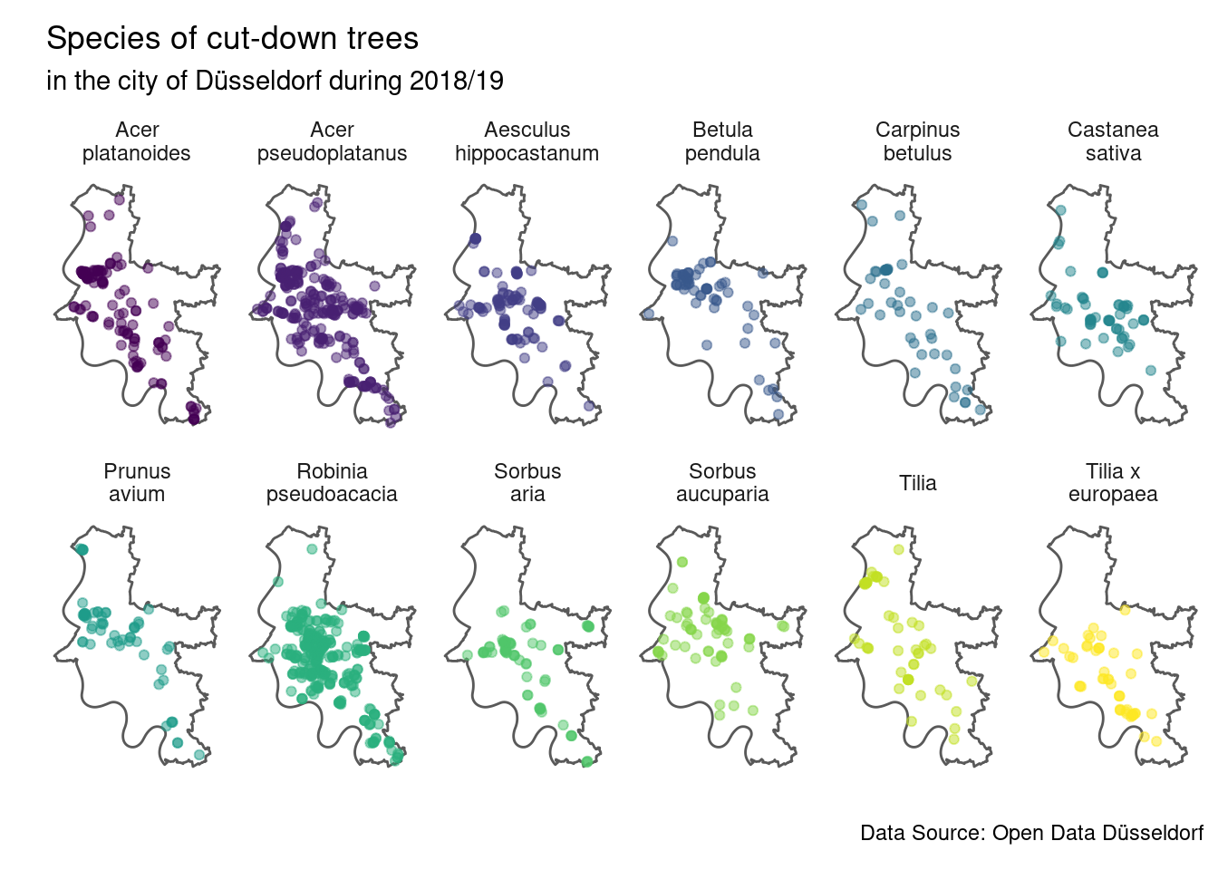

Most species of trees that were cut-down are more or less distributed over the entire city, with the exceptions being Sorbus aria and Tilia x europaea which were not cut-down in the north. It is important to note that we can not conclude that those two trees are absent or rare in northern parts of the city, only that they were not cut-down in these places.

To finish things let’s pick two species and have a look at the reasons they were cut down. We choose Acer platanoides and Sorbus aucuparia, but this is pretty random.

trees_2 <- trees_common %>% 
  filter(species %in% c("Acer platanoides", "Sorbus aucuparia"))

This leaves us with a relatively small selection of data.

nrow(trees_2)

## [1] 181

Again, extract the reasons for cutting-down.

trees_2_reasons <- reasons_long_data(trees_2, id, lat, lon, species, quarter)

So we can now look at the reasons for cutting the trees down. As the numbers become really low really fast we only consider the top 5 reasons.

t2_reason_counts <- trees_2_reasons %>% 
  add_count(species, reason, sort = TRUE) %>% 
  select(species, reason, n) %>% 
  distinct() %>% 
  group_by(species) %>% 
  group_split() %>% 
  purrr::map(function(x) x %>% mutate(n = n / sum(n)) %>% slice(1:5))

t2_reason_counts

## [[1]]
## # A tibble: 5 x 3
##   species          reason             n
##   <chr>            <chr>          <dbl>
## 1 Acer platanoides other_or_none 0.523 
## 2 Acer platanoides dead          0.277 
## 3 Acer platanoides trunkdamage   0.0773
## 4 Acer platanoides rot           0.0409
## 5 Acer platanoides fungus        0.0409
## 
## [[2]]
## # A tibble: 5 x 3
##   species          reason             n
##   <chr>            <chr>          <dbl>
## 1 Sorbus aucuparia other_or_none 0.508 
## 2 Sorbus aucuparia dead          0.262 
## 3 Sorbus aucuparia fungus        0.177 
## 4 Sorbus aucuparia trunkdamage   0.0231
## 5 Sorbus aucuparia rot           0.0154

This data suggests that fungus infections are more common in Sorbus aucuparia than in Acer platanoides.

We can evaluate this more systematically by calculating a Chi-Square test:

t2_chsq <- table(trees_2_reasons$species, trees_2_reasons$reason) %>% 
  chisq.test()

broom::tidy(t2_chsq)

## # A tibble: 1 x 4
##   statistic p.value parameter method                    
##       <dbl>   <dbl>     <int> <chr>                     
## 1      26.2 0.00186         9 Pearson's Chi-squared test

This does suggest there are differences, but of course that lacks information on where the differences are.

Fortunately we can look a the standardised residuals of the test to get more information and then make an informed decision.

t2_chsq$stdres %>% 
  as_tibble(.name_repair = ~ c("species", "reason", "stdres")) %>% 
  filter(abs(stdres) > 2)

## # A tibble: 4 x 3
##   species          reason      stdres
##   <chr>            <chr>        <dbl>
## 1 Acer platanoides fungus       -4.27
## 2 Sorbus aucuparia fungus        4.27
## 3 Acer platanoides trunkdamage   2.11
## 4 Sorbus aucuparia trunkdamage  -2.11

We see potential differences for trunk damage and fungus. However for trunk damage we see that the standardised residual is not that big, while it is considerably larger for fungus.

So we carefully conclude that Sorbus aucuparia had to be cut down in 2018/19 in Düsseldorf more often due to fungus infection than Acer platanoides. This might be due to the Sorbus aucuparia being more vulnerable to fungi, but this might as well be just a random pattern in the data.

To wrap things up we can plot the reasons for cutting down these two species of trees.

trees_2_reasons %>% 
  mutate(reason = gsub("_or_", "/", .$reason)) %>% 
  group_by(reason) %>% 
  add_count() %>% 
  ungroup() %>% 
  filter(n >= 5) %>% 
  ggplot() +
    geom_sf(data = dus_city, fill = "white") +
    geom_point(aes(x = lon, y = lat, colour = reason), alpha = 0.5) +
    scale_colour_viridis_d() +
    guides(colour = FALSE) +
    facet_grid(species~reason, switch = "y") +
    coord_sf(datum = NA) +
    theme_minimal() +
    labs(x = "", y = "", 
         title = paste("Reasons for cutting down",
                       "Acer plantanoides and Sorbus aucuparia"),
         subtitle = "in the city of Düsseldorf during 2018/19",
         caption = source_str)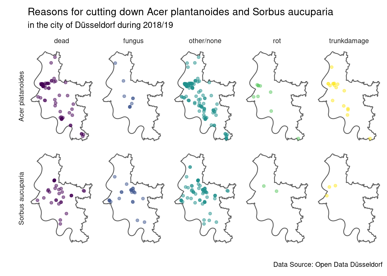

It seems like for Sorbus aucuparia there is one cluster of fungus infections (a bit north-east of the centre), which might explain the results from the Chi-Square test at least a bit. As the test also suggested we do see quite a bit of trunk damage for Acer plantanoides across large parts of the city. But note that the visual comparison alone is a bit difficult due to varying sizes of the groups (there are more Acer plantanoides than Sorbus aucuparia overall).

Conclusions

• Where the reasons are known trees are generally cut-down for good reasons.
• However there is a large fraction of unknown reasons, so the city should improve its data gathering and standardisation.
• The lack of standardisation is also striking with the species of trees, for many names there are several variants for the spelling, but it seems like something that can easily be standardised (even with a spreadsheet)
• Unfortunately data on all trees in the city is not available, the same is true for data on newly planted trees. Analysing cut-down trees together with the overall trees in the city would really be interesting and would enable much more meaningful conclusions.

So at the end we got some information about trees that were cut-down in Düsseldorf, Germany based on open data published by the city. The analysis is nothing too fancy (again mostly due to the fact that there is no data on all trees), but it was nice exploring the dataset.