Research papers

Fortunately, the idea of open-access publishing has become established during the past decade, so a large amount of papers are available online without restrictions.

I decided to use the Frontiers family of journals as data source, mainly for two reasons: 1. they have a wide variety of disciplines in distinct journals; 2. the URLs and DOIs of the papers are fully predictable, including an abbreviation for the journal title, the year and a counter.

Scraping the Frontiers website was an easy way to get considerable amounts of full text papers for a defined discipline and year (also, they explicitly allow scraping in their terms of service as of the time of writing).

A total of 4500 URLs were scraped for potential candidate papers, from three disciplines (neurosicence, psychology and physiology) over three years (2016-2018) using the first 500 numbers per year. The final dataset included 2551 papers.

What happened to the remaining 2000 papers? There is a variety of reasons that they were not included in the final dataset: Some URLs did not return a result, some were very brief texts (most likely things like commentary and correction articles) and some were lost during processing.

I tried to split the texts into the standard sections of a scientific paper, namely Introduction, Methods, Results and Discussion. Papers were lost here due to using non-standard section headings, which is often the case with review papers, but sometimes also happens with regular papers.

After scraping and cleaning the data looked like this:

# Random example
paperlist[[4]][[17]]

## # A tibble: 66 x 4
##    id       doi             section   text                                 
##    <chr>    <chr>           <chr>     <chr>                                
##  1 fpsyg_2… 10.3389/fpsyg.… Introduc… It is well known that the time requi…
##  2 fpsyg_2… 10.3389/fpsyg.… Introduc… Given that no controversy exists on …
##  3 fpsyg_2… 10.3389/fpsyg.… Introduc… Alternatively, it has been argued th…
##  4 fpsyg_2… 10.3389/fpsyg.… Introduc… If we narrow the discussion down to …
##  5 fpsyg_2… 10.3389/fpsyg.… Introduc… Evidence has also been reported of a…
##  6 fpsyg_2… 10.3389/fpsyg.… Introduc… Despite these differences, some proc…
##  7 fpsyg_2… 10.3389/fpsyg.… Introduc… The converging anatomical substrate …
##  8 fpsyg_2… 10.3389/fpsyg.… Introduc… As noted above, picture naming and w…
##  9 fpsyg_2… 10.3389/fpsyg.… Introduc… According to the theoretical account…
## 10 fpsyg_2… 10.3389/fpsyg.… Methods   The present study was approved by th…
## # … with 56 more rows

Citation data

For citation data I used the CrossRef API as implemented in the rcrossref package. To get metadata for a paper you need the DOI, short for document object identifier, an unique ID for various materials commonly used for research papers.

When querying the API for a specific DOI you get a bunch of information about the work in question, including the number of works that are referencing it (i.e. the number of times a work has been cited at the time of querying).

As the DOIs for Frontiers papers are rather easy to derive from the URLs, I just added them to the scraped data. In the next step, I then called the CrossRef API and extracted the is-referenced-by-count item from the returned data

The result from this step looked like this:

citation_numbers

## # A tibble: 3,213 x 2
##    doi                      citations
##    <chr>                        <dbl>
##  1 10.3389/fnins.2016.00001         5
##  2 10.3389/fnins.2016.00004        17
##  3 10.3389/fnins.2016.00006         4
##  4 10.3389/fnins.2016.00007         2
##  5 10.3389/fnins.2016.00008         9
##  6 10.3389/fnins.2016.00009         4
##  7 10.3389/fnins.2016.00010         2
##  8 10.3389/fnins.2016.00011        35
##  9 10.3389/fnins.2016.00014        23
## 10 10.3389/fnins.2016.00015         1
## # … with 3,203 more rows

It is pretty obvious that it is easy to merge this data with the text extracted from the papers as shown above.

Sentiment data

The remaining ingredient for this analysis is data on the sentiment of words, i.e. whether a word has a positive or negative connotation. I used the AFINN dictionary as it contains not only a general characterisation of the sentiment, but also a quantification of it. The AFINN data can be accessed easily using tidytext::get_sentiments() and it looks like this:

afinn

## # A tibble: 2,477 x 2
##    word       value
##    <chr>      <dbl>
##  1 abandon       -2
##  2 abandoned     -2
##  3 abandons      -2
##  4 abducted      -2
##  5 abduction     -2
##  6 abductions    -2
##  7 abhor         -3
##  8 abhorred      -3
##  9 abhorrent     -3
## 10 abhors        -3
## # … with 2,467 more rows

The higher a negative value (i.e. the father away from 0) the more negative is the sentiment of a word and the opposite is true for positive values and their associated sentiment.

Putting it all together

For being able to classify the words from the papers according to this dictionary, it was necessary to first tokenise the raw text data. This means to put each word in its own row, to convert the spelling to lower case and to remove all punctuation. There is the tidytext::unnest_tokens() function to do this rather conveniently. The text then looks like this:

papertbl

## # A tibble: 16,106,947 x 4
##    id         doi                      section      word          
##    <chr>      <chr>                    <chr>        <chr>         
##  1 fnins_2016 10.3389/fnins.2016.00001 Introduction neurocognitive
##  2 fnins_2016 10.3389/fnins.2016.00001 Introduction studies       
##  3 fnins_2016 10.3389/fnins.2016.00001 Introduction employ        
##  4 fnins_2016 10.3389/fnins.2016.00001 Introduction experimental  
##  5 fnins_2016 10.3389/fnins.2016.00001 Introduction manipulation  
##  6 fnins_2016 10.3389/fnins.2016.00001 Introduction of            
##  7 fnins_2016 10.3389/fnins.2016.00001 Introduction variables     
##  8 fnins_2016 10.3389/fnins.2016.00001 Introduction such          
##  9 fnins_2016 10.3389/fnins.2016.00001 Introduction as            
## 10 fnins_2016 10.3389/fnins.2016.00001 Introduction attention     
## # … with 16,106,937 more rows

You can see that this data structure is rather big with over 16 million rows.

Given the structure of the data containing the tokenised text and the structure of the sentiment data, it can be easily combined using dplyr::inner_join(). The data then looks like this:

papertbl_sen

## # A tibble: 498,997 x 5
##    id         doi                      section      word         value
##    <chr>      <chr>                    <chr>        <chr>        <dbl>
##  1 fnins_2016 10.3389/fnins.2016.00001 Introduction manipulation    -1
##  2 fnins_2016 10.3389/fnins.2016.00001 Introduction error           -2
##  3 fnins_2016 10.3389/fnins.2016.00001 Introduction ensure           1
##  4 fnins_2016 10.3389/fnins.2016.00001 Introduction capable          1
##  5 fnins_2016 10.3389/fnins.2016.00001 Introduction innovative       2
##  6 fnins_2016 10.3389/fnins.2016.00001 Introduction innovative       2
##  7 fnins_2016 10.3389/fnins.2016.00001 Introduction manipulation    -1
##  8 fnins_2016 10.3389/fnins.2016.00001 Introduction luck             3
##  9 fnins_2016 10.3389/fnins.2016.00001 Introduction stimulating      2
## 10 fnins_2016 10.3389/fnins.2016.00001 Introduction problems        -2
## # … with 498,987 more rows

Two things are apparent: 1. the data has been reduced quite dramatically from over 16 million rows to about 500,000; 2. each row now has a sentiment characterisation in the value column.

To answer the initial question two things remain to be done, first summarise the data per paper (getting mean, standard deviation and amount of words with sentiment per paper).

paper_sen <- papertbl_sen %>%
    dplyr::group_by(doi, section) %>%
    dplyr::summarise(mean = mean(value), sd = sd(value), count = n()) %>%
    dplyr::filter(n() == 4)

The last line filters the data so only those rows are kept where sentiment data is present for all four sections of an article.

Then while we are at it transform the section column to factor type, to keep the sections in the same order as they usually appear in a paper (this is useful when plotting):

paper_sen <- dplyr::mutate(paper_sen, section = factor(section,
    levels = c("Introduction", "Methods", "Results", "Discussion")))

Finally, we can add data on journal and year back to the now summarised data as well as adding citation information.

id_doi <- papertbl %>%
    dplyr::select(id, doi) %>%
    dplyr::distinct()

paper_sen <- dplyr::inner_join(paper_sen, citation_numbers)
paper_sen <- dplyr::inner_join(paper_sen, id_doi)
paper_sen <- tidyr::separate(paper_sen, id,
                             into = c("journal", "year"), sep = "_")

Now, the data looks like this:

paper_sen

## # A tibble: 10,228 x 8
## # Groups:   doi [2,557]
##    doi               section       mean    sd count citations journal year 
##    <chr>             <fct>        <dbl> <dbl> <int>     <dbl> <chr>   <chr>
##  1 10.3389/fnins.20… Discussion  0.513   1.65    76         5 fnins   2016 
##  2 10.3389/fnins.20… Introduct…  0.7     1.59    20         5 fnins   2016 
##  3 10.3389/fnins.20… Methods     0.169   1.75    59         5 fnins   2016 
##  4 10.3389/fnins.20… Results     1.21    1.90    34         5 fnins   2016 
##  5 10.3389/fnins.20… Discussion  0.0556  1.80    36        17 fnins   2016 
##  6 10.3389/fnins.20… Introduct… -0.412   1.80    17        17 fnins   2016 
##  7 10.3389/fnins.20… Methods    -0.259   1.48    27        17 fnins   2016 
##  8 10.3389/fnins.20… Results    -0.393   1.31    28        17 fnins   2016 
##  9 10.3389/fnins.20… Discussion  0.714   1.41    35         4 fnins   2016 
## 10 10.3389/fnins.20… Introduct…  0.824   1.42    34         4 fnins   2016 
## # … with 10,218 more rows

Given how the data was prepared we can now proceed to plot citations by sentiment also including information about the journal (essentially being a representation of the scientific discipline) and the year a paper was published in:

ggplot(paper_sen) +
  aes(x = mean, y = citations, colour = year) +
  geom_vline(xintercept = 0, colour = "grey40") +
  geom_point(alpha = .5) +
  facet_grid(section~journal) +
  labs(x = "Mean Sentiment", y = "Number of Citations",
       colour = "Year of\nPublication")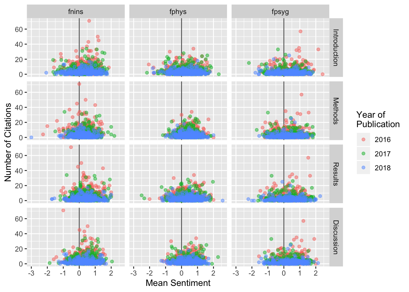

From the plot we can see two things: 1. there seems to be no strong relationship between citations and sentiment of the text of a paper; 2. older papers appear to be cited more often, which is straightforward as they have been available for longer time. It further appears like there are no obvious trends across the standard sections of a paper.

While the plot already strongly suggests that there is no relationship between sentiment and amount of citations, let’s look look at the correlation between both values:

cor(paper_sen$citations, paper_sen$mean)

## [1] 0.03093981

With a correlation of this size it is safe to say that there is no relationship.

Finally, we can also look at the mean values for sentiment for the individual sections:

papertbl_sen %>% 
  group_by(section) %>% 
  summarise(mean = mean(value), sd = sd(value))

## # A tibble: 4 x 3
##   section       mean    sd
##   <chr>        <dbl> <dbl>
## 1 Discussion   0.366  1.74
## 2 Introduction 0.266  1.81
## 3 Methods      0.253  1.68
## 4 Results      0.311  1.63

And without splitting into sections:

papertbl_sen %>% 
    summarise(mean = mean(value), sd = sd(value))

## # A tibble: 1 x 2
##    mean    sd
##   <dbl> <dbl>
## 1 0.303  1.73

From this we can see that the mean values are slightly into the range of positive sentiments, but the standard deviations are so large that most papers are in a reasonable range around 0.

This is very good news, as the near-zero correlation suggests that overall it does not matter whether a paper is written more positively or negatively.