Euclidean distance

To characterise how close an observation is to another you need some sort of distance metric. A very popular metric here is the Euclidean Distance, a relatively simple, but nonetheless effective and useful characterisation of distance. Consider the following matrix:

mt <- matrix(c(1, 1, 10, 10), ncol = 2, byrow = TRUE)
mt

##      [,1] [,2]
## [1,]    1    1
## [2,]   10   10

We want to calculate the distance between rows. Euclidean distance is the square root of the sum of squares of the differences between the rows, or to show it with the actual numbers:

sqrt(sum(c(((1 - 10) ^ 2), ((1 - 10) ^ 2))))

## [1] 12.72792

We can verify this by using R’s built-in distance function, dist:

dist(mt)

##          1
## 2 12.72792

However, in the from scratch series we want to implement things ourselves. Let’s return to our example data first. Doing operations on vectors is easy in R and one of the strong points of the language.

sqrt(sum((mt[1, ] - mt[2, ]) ^ 2))

## [1] 12.72792

So we just need to do that calculation for all rows in our data, in case we deal with something bigger than a 2 by 2 matrix, right? Right.

euclidean_dist <- function(data) {
    distances <- apply(data, 1, function(x) {
        apply(data, 1, function(y) {
            sqrt(sum((x - y) ^ 2))
        })
    })
    distances
}

The nested apply structure ensures that we work on all possible pairs of rows and is more or less the equivalent of nested for loops in other languages. Now, you might be thinking that this approach is not super-efficient and you are correct. For any given pair of rows the distance will be calculated twice and we should subset the data before the inner apply and adapt our output if this was more than a toy example for learning.

When we calculate Euclidean distance between all observations (rows) of a data set we can find which are the closest observations either to each other, or to some reference, as some distances might turn out to be relatively small, some might be larger.

The curse of dimensionality

As mentioned above, there is a phenomenon related to finding groups in data that is known as the curse of dimensionality. This phenomenon encompasses that with very high-dimensional data (think for example 100 columns) it becomes very hard to successfully find groups in data. Looking at how we calculate Euclidean distance it is easy to see why this is the case. Unless your data is as clean as data found in textbooks the amount of noise and variance in the columns will eventually lead to distances becoming less selective and distinct. As far as I can see there is no magic number where the curse of dimensionality begins, but if you want to cluster using many columns, chances are that you are affected by it.

Clustering

Now that we have established how to characterise the distance between observations, we can move on to clustering. This is actually pretty easy in the case of k-means:

1. Randomly select k distinct observations from the data to use as cluster centres.
2. Calculate the distances between the cluster centres and all data points.
3. Find which of the k observations is the closest and label the data accordingly.
4. For each group find the column means and use these as the new cluster centres.
5. Repeat steps 2, 3 and 4 until the cluster centres do not change any more or a maximum number of iterations has been reached.

That does not sound too complex, doesn’t it? Despite the relative simplicity the approach does work reasonably well, although there are datasets that it fails on quite spectacularly.

Let’s look at the code.

First we need some example data and set the amount of clusters we want to find. The iris dataset might serve as a nice example here, as it is commonly used as an example dataset for clustering. To ensure that a single column has not too much influcence on the distance metric, the data is scaled as well. We also set a seed for reproducibility.

set.seed(42)
data(iris)
data <- scale(iris[, 1:4]) # omit the labels
k <- 3

First we draw a random sample of size k, and create two matrices: one with our centres we just selected, the other to later use for the updated values, which we can then compare to the previous one to see whether they are still changing.

center_idx <- sample(1:nrow(data), k)
centers <- data[center_idx, ]
center_mean <- as.data.frame(matrix(NA, ncol = ncol(centers),
                                    nrow = nrow(centers)))
centers

##      Sepal.Length Sepal.Width Petal.Length   Petal.Width
## [1,]   -0.6561473   1.4744583  -1.27910398 -1.3110521482
## [2,]   -0.2938574  -0.3609670  -0.08950329  0.1320672944
## [3,]    0.3099591  -0.5903951   0.53362088  0.0008746178

The next steps are straightforward. When putting things together later on these will be enclosed in a while loop. But to have a look at the intermediate steps, we do one iteration manually.

The first step is calculating the distance between our initial selection and all observations.

distances <- euclidean_dist(rbind(centers, data))

If we take all but the first k rows and only the first k columns we have the distances of all observations to the cluster centres.

kdist <- distances[-c(1:k), 1:k]
head(kdist)

##           [,1]     [,2]     [,3]
## [1,] 0.5216255 2.428017 3.041925
## [2,] 1.6780274 2.098326 2.743414
## [3,] 1.3615373 2.331341 3.021808
## [4,] 1.6154093 2.273031 2.960103
## [5,] 0.4325508 2.596145 3.217006
## [6,] 0.5539087 2.806177 3.327659

As each column in our sub-setted distance matrix contains the distance to each of the cluster centres we can determine which cluster each observation is the closest to. Note that which.min returns only the first extreme observation in case of ties.

labels <- as.factor(apply(kdist, 1, which.min))
names(labels) <- NULL
head(labels)

## [1] 1 1 1 1 1 1
## Levels: 1 2 3

Now that each observation is associated with a cluster we can update the means of the clusters. The function by is the equivalent in base R for the group_by() %>% summarise() %>% ungroup() schema in dplyr. You supply a dataset, a grouping vector and a function you want to apply to each group. As the function returns a list, we bind it together using rbind with do.call.

center_mean <- by(data, labels, colMeans)
center_mean <- do.call(rbind, center_mean)
center_mean

##   Sepal.Length Sepal.Width Petal.Length Petal.Width
## 1   -0.9987207   0.9032290  -1.29875725 -1.25214931
## 2   -0.4593478  -0.8623100   0.09092997  0.09319539
## 3    0.8289150  -0.2834575   0.82681076  0.79512217

What’s left is checking whether our new centres are equivalent to our previous centres. If yes, we would leave our while loop on finishing the iteration, if not we would continue. No matter what we do, we update the centers variable first. Note, that while our first selection of centres corresponded to actual data points in the data, after the first update it is likely that they are in-between data-points.

if (all(center_mean == centers)) {
    not_converged <- FALSE
}
centers <- center_mean

So, now that we went through all the steps once, we can put this together into a function:

k_means <- function(data, k, max_iterations = 100) {
    center_idx <- sample(1:nrow(data), k)
    centers <- data[center_idx, ]
    center_mean <- as.data.frame(matrix(NA, ncol = ncol(centers),
                                        nrow = nrow(centers)))

    not_converged <- TRUE
    iter_count <- 1

    while (not_converged) {
        distances <- euclidean_dist(rbind(centers, data))
        kdist <- distances[-c(1:k), 1:k]
        labels <- as.factor(apply(kdist, 1, which.min))
        names(labels) <- NULL

        center_mean <- by(data, labels, colMeans)
        center_mean <- do.call(rbind, center_mean)

        if (all(center_mean == centers)) {
            not_converged <- FALSE
        }
        centers <- center_mean
        iter_count <- iter_count + 1
        if (iter_count > max_iterations) {
            warning("Did not converge.")
            break()
        }
    }

    list(labels = labels, centers = centers, iterations = iter_count)
}

Note a few additions here:

• As mentioned we added a while loop that ends once our centres do not update any more.
• Also, we have added a counter for iterations and another condition for breaking out of our while loop. This is not ensure that you are not stuck in an endless-loop, but also to ensure that you are not over-optimising. The case that k-means takes 100 iterations to produce usable results is pretty rare, usually it converges rather fast.
• At the end we return a list containing our labels, the centres and the iterations it took us before converging.

Now let’s give this a try:

km <- k_means(data, 3)

And have a look at whether we were able to separate the iris species.

table(km$labels, iris$Species)

##    
##     setosa versicolor virginica
##   1      0         11        36
##   2      0         39        14
##   3     50          0         0

And plot it (we have four dimensions, so we choose only two for siplicity).

library("ggplot2")
ggplot(iris) + 
  aes(x = Sepal.Width, y = Petal.Length) +
  geom_point(aes(colour = km$labels))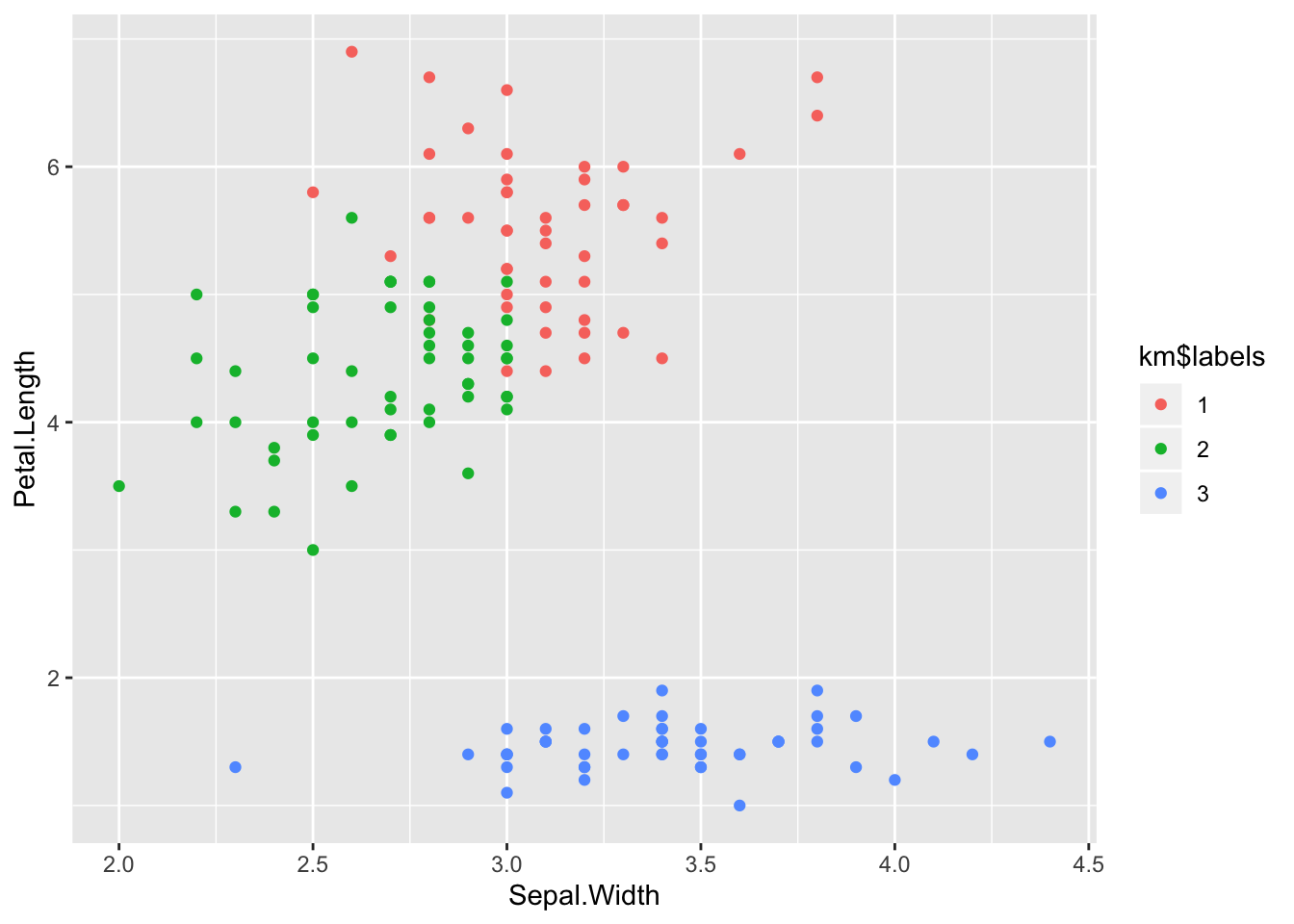

Apparently there is some confusion between versicolor and viriginica, but the result are not too bad. Compare with stats::k-means.

km2 <- kmeans(data, 3)
table(km2$cluster, iris$Species)

##    
##     setosa versicolor virginica
##   1      0         46        50
##   2     33          0         0
##   3     17          4         0

ggplot(iris) + 
  aes(x = Sepal.Width, y = Petal.Length) +
  geom_point(aes(colour = as.factor(km2$cluster)))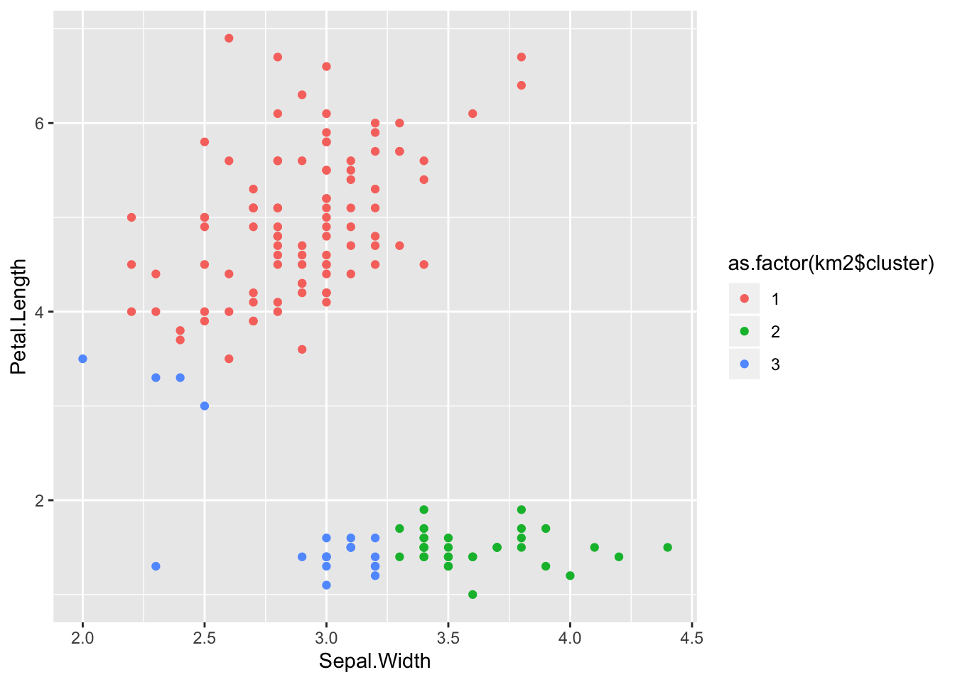

The results we got here are even worse. While k-means is pretty elegant and works reasonably well, it is very dependant on the initial selection of cluster centres. Thus, it can end up in a local best solution, which is not necessarily the best available solution. The stats stats::k-means has the argument nstart which aims to mitigate this situation by trying several initial selections and returning the best result only.

km3 <- kmeans(data, 3, nstart = 10)
table(km3$cluster, iris$Species)

##    
##     setosa versicolor virginica
##   1      0         11        36
##   2      0         39        14
##   3     50          0         0

ggplot(iris) + 
  aes(x = Sepal.Width, y = Petal.Length) +
  geom_point(aes(colour = as.factor(km3$cluster)))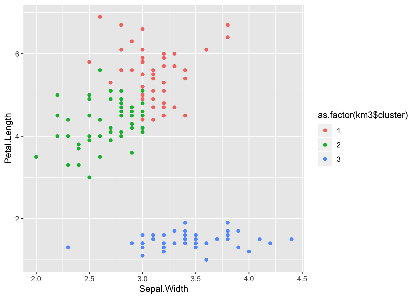

Which is still not perfect (and very similar to what we got with our own implementation), but there is only so much you can do.

Conclusions

Doing a basic implementation of k-means was a nice learning experience. We have seen that at its core the method is quite simple, but nonetheless is able to provide useful results.

Additionally, the Gitlab repo for the fromscratch package also contains implementations of both k-means and euclidean distance in C++. Writing the C++ implementation was much harder than the R version, but at the end the C++ version runs considerably faster.

And finally, note that there are several variations available on how to implement the clustering, as reflected by the algorithm option in stats::kmeans.