Formula parsing

Let me start by stating that paring of formulae in R is pretty painful and that I am a bit surprised that given the popularity of the formula interface the tools available to extract information from them appear a bit inconvenient.

The following is the code I used, where data is the input data and f the formula passed to the function.

f_details <- terms(f)
pred_order <- attr(f_details, "order")
pred_names <- attr(f_details, "term.labels")
x_names <- unique(unlist(strsplit(pred_names, "[[:punct:]]")))
x_vars <- pred_names[pred_order == 1]
f_allvars <- all.vars(f_details)
y_names <- f_allvars[!f_allvars %in% x_names]

xdata <- data[, x_vars]

if (attr(f_details, "intercept") == 1) {
    xdata[["intercept"]] <- 1
}

if (any(pred_order > 1)) {
    i_labels <- pred_names[pred_order > 1]
    i_vars <- sapply(i_labels, strsplit, ":", USE.NAMES = FALSE)
    for (term in i_vars) {
        prod_var <- rep(1, times = nrow(xdata))
        prod_name <- paste(term, collapse = ":", sep = "")
        for (v in term) {
            prod_var <- prod_var * data[, v]
        }
        xdata[prod_name] <- prod_var
    }
}

ydata <- data[, y_names]

First we look at the parts of the formula to find out what is in there and then create subsets of the input data for the response (ydata) and the predictors (xdata). We try to find interactions in the formula (mainly looking for the : sign in the names of the factors attribute, if you specify an interaction as a * b, this will be automatically expanded to a + b + a:b) and add columns to xdata as needed. This can handle interactions, but won’t properly deal with factors or things like as.numeric(var) as part of the formula.

You can use the terms function to extract information from a formula; it will return the formula and numerous attributes.

terms(y ~ x1 + x2)

## y ~ x1 + x2
## attr(,"variables")
## list(y, x1, x2)
## attr(,"factors")
##    x1 x2
## y   0  0
## x1  1  0
## x2  0  1
## attr(,"term.labels")
## [1] "x1" "x2"
## attr(,"order")
## [1] 1 1
## attr(,"intercept")
## [1] 1
## attr(,"response")
## [1] 1
## attr(,".Environment")
## <environment: R_GlobalEnv>

While on the one hand this contains everything you need, on the other hand this requires that you have a good idea of what potentially to expect and having a way to handle it all. The above call was relatively simple, but things can be much more complex.

terms(y ~ 0 + x1 + x2 + x1:x3:x4)

## y ~ 0 + x1 + x2 + x1:x3:x4
## attr(,"variables")
## list(y, x1, x2, x3, x4)
## attr(,"factors")
##    x1 x2 x1:x3:x4
## y   0  0        0
## x1  1  0        2
## x2  0  1        0
## x3  0  0        2
## x4  0  0        2
## attr(,"term.labels")
## [1] "x1"       "x2"       "x1:x3:x4"
## attr(,"order")
## [1] 1 1 3
## attr(,"intercept")
## [1] 0
## attr(,"response")
## [1] 1
## attr(,".Environment")
## <environment: R_GlobalEnv>

Here we have no intercept and a 3rd order interaction involving two variables that are otherwise not part of the formula. Handling this is not impossible, but a bit tedious. I wish there were nicer tools available to handle formulae out of the box.

Linear regression with code

For a detailed walk-through with maths I suggest you have a look at the Linear Regression and Least Squares section in Elements of Statistical Learning. This is a great book and you can even download it for free, which is very nice (but consider buying it to support the authors’ work).

Linear regression boils down to the following:

response <- intercept + beta_1 * predictor_1 + beta_k * predictor_k

Where you can have as many predictors as you like. Here, predictors would be vectors (this includes columns of data frames and matrices), while the intercept and beta values would be scalars (a single numeric value). The prediction you get out of this is of course also a vector.

Given that we know the predictors we want to use and also have an associated response to train our model the task is to find good values for the beta values. This is what least squares is used for, here you want to minimise the overall distance between the regression line (your predicted response) and the actual data.

Let’s build a visual example.

set.seed(6578423) # for reproducibility
library("ggplot2")
d <- data.frame(x = rnorm(100), y = rnorm(100))
mod <- lm(y ~ x, data = d)
d$fit <- fitted(mod)
ggplot(d) +
    aes(x = x, y = y) +
    geom_point(color = "red") +
    geom_line(aes(y = fit), alpha = .8, size = 1.5) +
    geom_linerange(aes(ymin = y, ymax = fit), alpha = .8)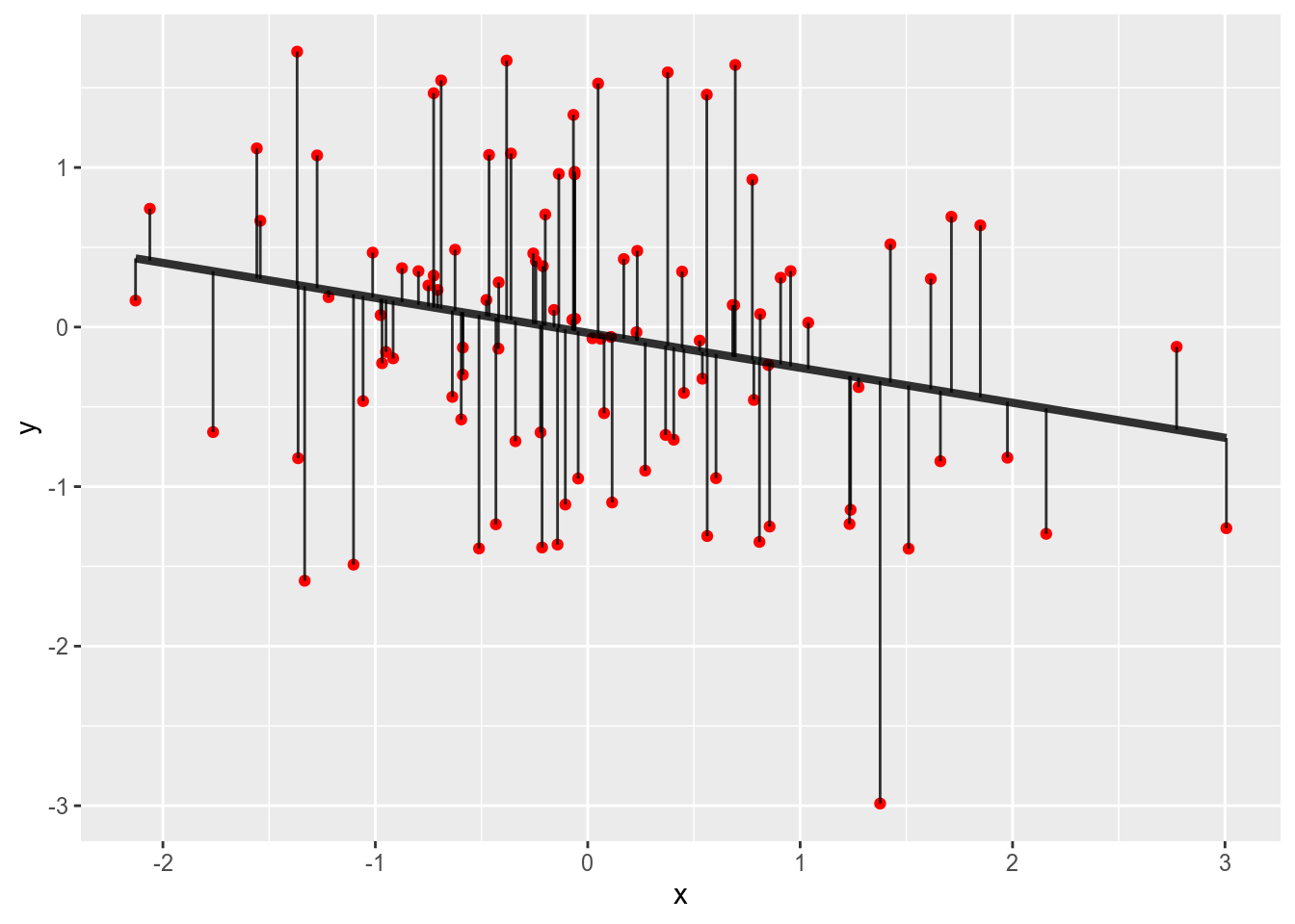

Our data are the red points with the vertical lines visualising the distance to the regression line. What we want is that the sum of squares of the length of the vertical lines is as small as possible. Given that we fitted the model with lm what we see here is in fact the smallest sum of squares of the distances for the given data.

From the equation above one can derive the calculation of the coefficients with ordinary least squares, which is as follows:

beta <- solve(t(xdata) %*% xdata) %*% t(xdata) %*% ydata

The function t gives the transpose of a matrix (rotation, so columns are now rows and vice versa), while solve called on a single matrix will return the matrix inverse. The operator %*% indicates matrix multiplication, if you use a regular * R will perform element-wise multiplication. Matrix inverses are really interesting matrices as multiplying a matrix with its inverse returns the identity matrix (a matrix with all 1 on the diagonal and 0 otherwise).

mx <- matrix(c(5, 7, 4, 9, 11, 8, 4, 16, 15), ncol = 3)
mx

##      [,1] [,2] [,3]
## [1,]    5    9    4
## [2,]    7   11   16
## [3,]    4    8   15

mi <- solve(mx)
mi

##             [,1]        [,2]        [,3]
## [1,] -0.27205882  0.75735294 -0.73529412
## [2,]  0.30147059 -0.43382353  0.38235294
## [3,] -0.08823529  0.02941176  0.05882353

mx %*% mi

##               [,1]         [,2]          [,3]
## [1,]  1.000000e+00 6.938894e-16 -7.771561e-16
## [2,] -2.220446e-16 1.000000e+00  4.440892e-16
## [3,] -2.220446e-16 5.551115e-17  1.000000e+00

There are some floating point errors in the above matrix, but generally we see the diagonal being all 1 and the rest being 0.

Now we should get some data, to work further through the calculations.

data(mtcars)
head(mtcars)

##                    mpg cyl disp  hp drat    wt  qsec vs am gear carb
## Mazda RX4         21.0   6  160 110 3.90 2.620 16.46  0  1    4    4
## Mazda RX4 Wag     21.0   6  160 110 3.90 2.875 17.02  0  1    4    4
## Datsun 710        22.8   4  108  93 3.85 2.320 18.61  1  1    4    1
## Hornet 4 Drive    21.4   6  258 110 3.08 3.215 19.44  1  0    3    1
## Hornet Sportabout 18.7   8  360 175 3.15 3.440 17.02  0  0    3    2
## Valiant           18.1   6  225 105 2.76 3.460 20.22  1  0    3    1

We use mpg as response, cyl and hp as predictors (ignoring that cyl is not continuous). Let’s extract the data we are interested in and add an intercept (otherwise we would imply that the regression line runs through x = 0, y = 0).

ydata <- mtcars[, "mpg"]
xdata <- mtcars[, c("cyl", "hp")]
xdata$intercept <- 1
xdata <- as.matrix(xdata)

Now, we should be able to put these matrices into our equation from above. We do this in two steps as it turns out that the matrix inverse of t(xdata) %*% xdata is useful for subsequent calculations.

xinv <- solve(t(xdata) %*% xdata)
beta <- xinv %*% t(xdata) %*% ydata
beta

##                 [,1]
## cyl       -2.2646936
## hp        -0.0191217
## intercept 36.9083305

Those are our beta weights. We can check against lm.

lmod <- lm(mpg ~ cyl + hp, data = mtcars)
summary(lmod)

## 
## Call:
## lm(formula = mpg ~ cyl + hp, data = mtcars)
## 
## Residuals:
##     Min      1Q  Median      3Q     Max 
## -4.4948 -2.4901 -0.1828  1.9777  7.2934 
## 
## Coefficients:
##             Estimate Std. Error t value Pr(>|t|)    
## (Intercept) 36.90833    2.19080  16.847  < 2e-16 ***
## cyl         -2.26469    0.57589  -3.933  0.00048 ***
## hp          -0.01912    0.01500  -1.275  0.21253    
## ---
## Signif. codes:  0 '***' 0.001 '**' 0.01 '*' 0.05 '.' 0.1 ' ' 1
## 
## Residual standard error: 3.173 on 29 degrees of freedom
## Multiple R-squared:  0.7407, Adjusted R-squared:  0.7228 
## F-statistic: 41.42 on 2 and 29 DF,  p-value: 3.162e-09

The values in the Estimate column are the same as what we have calculated above.

Great.

There are more columns in the above table though, which we also might want to calculate while we are implementing our linear regression. The next would be the standard error, which is certainly a useful value as it transports quite a bit of information about how close the data is to our model (on the scale of the data).

Looking in our favourite statistics textbook we see that the standard error here is the square root of the diagonal of the variance-covariance matrix. This means we need to compute the variance-covariance matrix first. Doing so requires several steps, but nothing absurdly complex, we need the variance estimate for which we need the residuals and degrees of freedom:

fitted <- as.vector(as.matrix(xdata) %*% beta)
residuals = as.vector(ydata - fitted)
df <- length(ydata) - ncol(xdata)
variance_est <- (1 / df) * sum(residuals ^ 2)
var_cov_mat <- xinv * variance_est

This means the standard errors are now available as

se_preds <- sqrt(diag(var_cov_mat))
se_preds

##        cyl         hp  intercept 
## 0.57588924 0.01500073 2.19079864

Now we have two of the four columns from above. So, next would be t-values. Fortunately we have everything we need to calculate t-values, we just need to put it together the right way.

tval <- beta / (sqrt(variance_est) * sqrt(diag(xinv)))
tval

##                [,1]
## cyl       -3.932516
## hp        -1.274718
## intercept 16.846975

Finally we just need the p-values. Obviously you should not rely on p-values too much, but they are nonetheless a useful statistic if not abused for binary classification into meaningful and meaningless.

pval <-  2 * pt(abs(tval[, 1]), df = df, lower.tail = FALSE)
pval

##          cyl           hp    intercept 
## 4.803752e-04 2.125285e-01 1.620660e-16

The pt function can only handle directed hypotheses, so you need to double the values for the two sided case. Given that you will likely get both positive and negative values from the previous calculation for t-values the easiest way to get correct results is to work with absolute values.

And after we came here we have now replicated the results table from summary.lm ourselves.

Putting it all together

After we went through all the individual pieces above, we might want to create our own custom linear model function. Here it is:

linear_model <- function(data, f) {
#' Fit linear Regression.
#'
#' @param data The input data.
#' @param f The formula specifing the model to fit.
#'
#' The formula should contain one dependent variable on the left hand side
#' and as many predictors as you like on the right hand side. Interactions
#' can be specified as well.
#'
#' @return A named list, containing `coefficients`: a data frame with
#' weights, standard errors, t and p values; `augmented`: the input data
#' expanded with fitted values and residuals as well as `vcv` the
#' variance-covariance matrix.
    f_details <- terms(f)
    pred_order <- attr(f_details, "order")
    pred_names <- attr(f_details, "term.labels")
    x_names <- unique(unlist(strsplit(pred_names, "[[:punct:]]")))
    x_vars <- pred_names[pred_order == 1]
    f_allvars <- all.vars(f_details)
    y_names <- f_allvars[!f_allvars %in% x_names]

    xdata <- data[, x_vars]

    if (attr(f_details, "intercept") == 1) {
        xdata[["intercept"]] <- 1
    }

    if (any(pred_order > 1)) {
        i_labels <- pred_names[pred_order > 1]
        i_vars <- sapply(i_labels, strsplit, ":", USE.NAMES = FALSE)
        for (term in i_vars) {
            prod_var <- rep(1, times = nrow(xdata))
            prod_name <- paste(term, collapse = ":", sep = "")
            for (v in term) {
                prod_var <- prod_var * data[, v]
            }
            xdata[prod_name] <- prod_var
        }
    }

    ydata <- data[, y_names]

    xtx_inv <- solve(t(xdata) %*% as.matrix(xdata))

    coefs <-  xtx_inv %*% t(xdata) %*% as.matrix(ydata)
    results_coefs <- coefs[, 1]

    fitted <- as.vector(as.matrix(xdata) %*% coefs)
    residuals = as.vector(ydata - fitted)

    df <- length(ydata) - ncol(xdata)
    variance_est <- (1 / df) * sum(residuals ^ 2)
    var_cov_mat <- xtx_inv * variance_est
    se_preds <- sqrt(diag(var_cov_mat))

    tval <- coefs / (sqrt(variance_est) * sqrt(diag(xtx_inv)))

    results_tbl <- data.frame(
        predictor = names(results_coefs),
        coef = results_coefs,
        se = se_preds,
        t = tval[, 1],
        p = 2 * pt(abs(tval[, 1]), df = df, lower.tail = FALSE),
        stringsAsFactors = FALSE,
        row.names = NULL
    )

    data[[".fitted"]] <- fitted
    data[[".residuals"]] <- residuals

    list(coefficients = results_tbl,
         augmented = data,
         vcv = var_cov_mat)
}

You probably recognise many of the parts in this function from above. The first part is formula handling, before we calculate the values we are interested in and return some potentially useful information.

lmod_results <- linear_model(mtcars, mpg ~ hp + cyl)
lmod_results$coefficients

##   predictor       coef         se         t            p
## 1        hp -0.0191217 0.01500073 -1.274718 2.125285e-01
## 2       cyl -2.2646936 0.57588924 -3.932516 4.803752e-04
## 3 intercept 36.9083305 2.19079864 16.846975 1.620660e-16

The output here looks like we did everything correctly. Compare:

summary(lmod)

## 
## Call:
## lm(formula = mpg ~ cyl + hp, data = mtcars)
## 
## Residuals:
##     Min      1Q  Median      3Q     Max 
## -4.4948 -2.4901 -0.1828  1.9777  7.2934 
## 
## Coefficients:
##             Estimate Std. Error t value Pr(>|t|)    
## (Intercept) 36.90833    2.19080  16.847  < 2e-16 ***
## cyl         -2.26469    0.57589  -3.933  0.00048 ***
## hp          -0.01912    0.01500  -1.275  0.21253    
## ---
## Signif. codes:  0 '***' 0.001 '**' 0.01 '*' 0.05 '.' 0.1 ' ' 1
## 
## Residual standard error: 3.173 on 29 degrees of freedom
## Multiple R-squared:  0.7407, Adjusted R-squared:  0.7228 
## F-statistic: 41.42 on 2 and 29 DF,  p-value: 3.162e-09

The values in the tables are exactly the same.

C++

For some additional learning experience I also implemented the main parts of the above in C++. As you might know the Rcpp package provides an interface between R and C++ so you can write functions for R using C++. Functions you write in C++ are compiled (to machine code) before you can use them and are much faster compared to computations written purely in R. Thus, if you find yourself having serious requirements for high-performance code you might want to consider choosing this path as it might speed up your programs considerably.

Obviously C++ is a different language than R and getting up to speed might take a while if you have no or only little prior experience with C++. While having written code in many different programming languages before, my experience with C++ was very limited and such I learned quite a bit by also implementing linear regression in C++. I guess the most noteworthy difference when writing C++ compared to R is that the former is statically typed while the latter is dynamically typed. In R a variable is not bound to hold content of only one type, you can first assign a numeric value to a variable and later change it to a string. In C++ however you need to declare the type of a variable and the variable can then only contain data of that type. The approach in R gives more flexibility, but you need to be more careful when handling variables; while the approach in C++ is more rigid, but you can be sure what to expect.

Above, I stated that formula handling in R is more on the painful side of things. This is still true in my opinion, but I suppose handling formulae in C++ would be even worse, so while implementing linear regression in C++ I did handle the formula in R.

So, you can access the wrapper code here, which calls the core part as build in C++ (click this link for the code).

Before being able to use the function you need to compile it and to be able to compile it you need to set up the integration of C++ in R and also have a compiler installed. The usethis package can help you quite a bit with the whole set up and I suggest to have a look at its functions if you want to use C++ in your own packages.

Now, let’s call the C++ implementation:

lmod_c_results <- linear_model_cpp(mtcars, mpg ~ hp + cyl)
lmod_c_results$coefficients

##   predictor   estimate      error         t            p
## 1        hp -0.0191217 0.01500073 -1.274718 3.255820e-01
## 2       cyl -2.2646936 0.57588924 -3.932516 5.499192e-03
## 3 Intercept 36.9083305 2.19079864 16.846975 6.284157e-16

The results here are the same as with both other functions, suggesting that the implementation shown here is correct. Compare the results from our pure R implementation:

lmod_results$coefficients

##   predictor       coef         se         t            p
## 1        hp -0.0191217 0.01500073 -1.274718 2.125285e-01
## 2       cyl -2.2646936 0.57588924 -3.932516 4.803752e-04
## 3 intercept 36.9083305 2.19079864 16.846975 1.620660e-16

Conclusions

In this post we went through the inner workings of linear regression and build an implementation ourselves. Fortunately we got the same results as when calling lm.

We have seen that the core of the method is the calculation solve(t(xdata) %*% as.matrix(xdata)), which turns out to contain smaller values when the variance in the variables is greater, thus if there is a lot of variance in your data the coefficients will be smaller and the model fit worse.

Also, if you have ever seen error messages about a singular matrix when building a linear model, then the matrix inverse could not be computed (because there are linear dependencies in you data).

Finally, it has been an interesting and rewarding experience to build all this myself. Having the functions return the correct values for the first time (especially in case of the C++ function) was pretty neat and walking through the details of the method and the maths involved strengthened my understanding of it. As mentioned above, I am not the first person to build a function to fit a linear regression, but probably the end result was less relevant here than the path that lead to it.