Being able to generate colour palettes based on arbitrary images is quite useful if doing graphic design work of some kind.

Fortunately this can be done easily using R and relatively basic data science tools. In summary, you can take an image read it so you have the red, green and blue (RGB) colour channels separated and then apply k-means clustering to it. The nice thing about image data here is that with an image of reasonable size you easily get several million data points, so clustering works out nicely if you image is not just random noise.

Reading Images into R

For the most common image formats there are some handy packages, namely jpeg, png and tiff which are by the same author, so they pretty much work the same. They each provide a read function (readJPEG, readPNG, readTIFF) that returns a 3-dimensional array containing the image’s data. You then need to re-shape the data, cluster it and then you are almost done.

In Practice

So, let’s walk through an example image to demonstrate how to generate a colour palette from an image. The image we will be using can be found on Wikimedia Commons and it is in the Public Domain.

It looks like this: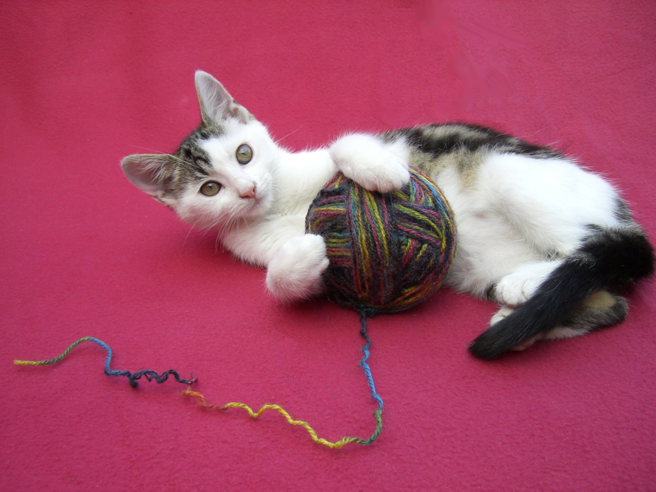

For the sake of readability I have renamed the file to playing_cat.jpg.

If you have the JPEG package installed it can be read easily into R.

library("jpeg")
fname <- "playing_cat.jpg"
img_data <- readJPEG(fname)

A quick look at the resulting data structure shows us that we got a 3d array with two dimensions being the axes of the image and the third dimension corresponding to RGB values.

dim(img_data)

## [1] 1920 2560    3

img_data[1, 1, ]

## [1] 0.5647059 0.1215686 0.2392157

With the three values above being the RGB representation of the pixel at position 1, 1.

To perform clustering on this data you need to reformat the data so it is a 2-dimensional structure. This can easily be accomplished with some simple looping over the data. Note that while for loops in R have a really bad reputation for being really slow, you can avoid the speed problem by not changing the size of the object you write to on the fly.

So, first generate an empty matrix of appropriate size:

rows_2d <- dim(img_data)[1] * dim(img_data)[2]
mx_2d <- matrix(NA, nrow = rows_2d, ncol = 5)

And then grab the data with two loops:

row_count <- 1

for (i in 1:dim(img_data)[1]) {
    for (j in 1:dim(img_data)[2]) {
        row <- c(i, j, img_data[i, j, 1],
                 img_data[i, j, 2], img_data[i, j, 3])
        mx_2d[row_count, ] <- row
        row_count <- row_count + 1
    }
}

On a somewhat recent machine this should complete within five seconds or so.

We can then proceed to transform the matrix to a data frame and column names and have a look at it.

mx_2d <- as.data.frame(mx_2d)
colnames(mx_2d) <- c("y", "x", "r", "g", "b")
head(mx_2d)

##   y x         r         g         b
## 1 1 1 0.5647059 0.1215686 0.2392157
## 2 1 2 0.5725490 0.1294118 0.2470588
## 3 1 3 0.5725490 0.1294118 0.2392157
## 4 1 4 0.5725490 0.1215686 0.2352941
## 5 1 5 0.5725490 0.1254902 0.2274510
## 6 1 6 0.5803922 0.1333333 0.2313725

This structure can easily be put into a clustering algorithm. Of course you do need to make sure that you do not include the x and y columns.

To use k-means:

km <- kmeans(mx_2d[, 3:5], centers = 5)
cluster_centres <- as.data.frame(km$centers)
cluster_centres

##           r         g         b
## 1 0.1637000 0.1028963 0.1139851
## 2 0.8929078 0.9026482 0.9016894
## 3 0.4225550 0.2663341 0.2851599
## 4 0.6984799 0.2228902 0.3734382
## 5 0.6623053 0.6094599 0.5957895

The output above are the mean points of the clusters, which represent the colours to use in our palette.

However, that representation is a bit abstract, so first we generate hexadecimal RGB names for our colours:

rgb <- apply(
    cluster_centres, 1, function(x) rgb(x[1], x[2], x[3]))
cluster_centres$rgb <- rgb
cluster_centres

##           r         g         b     rgb
## 1 0.1637000 0.1028963 0.1139851 #2A1A1D
## 2 0.8929078 0.9026482 0.9016894 #E4E6E6
## 3 0.4225550 0.2663341 0.2851599 #6C4449
## 4 0.6984799 0.2228902 0.3734382 #B2395F
## 5 0.6623053 0.6094599 0.5957895 #A99B98

These representations can then be used for plotting. Note the rgb function which is part of the grDevices package which is part of R itself (so you already have it).

Now visualise the colours:

library("ggplot2")
ggplot(cluster_centres) +
    aes(x = 1:nrow(cluster_centres), y = 1, fill = rgb) +
    geom_tile() +
    scale_fill_manual(values = cluster_centres$rgb) +
    scale_x_discrete(limits = cluster_centres$rgb) +
    theme_minimal() +
    labs(x = NULL, y = NULL) +
    theme(panel.grid = element_blank(),
          axis.line.y = element_blank(),
          axis.text.y = element_blank()) +
    guides(fill = "none")

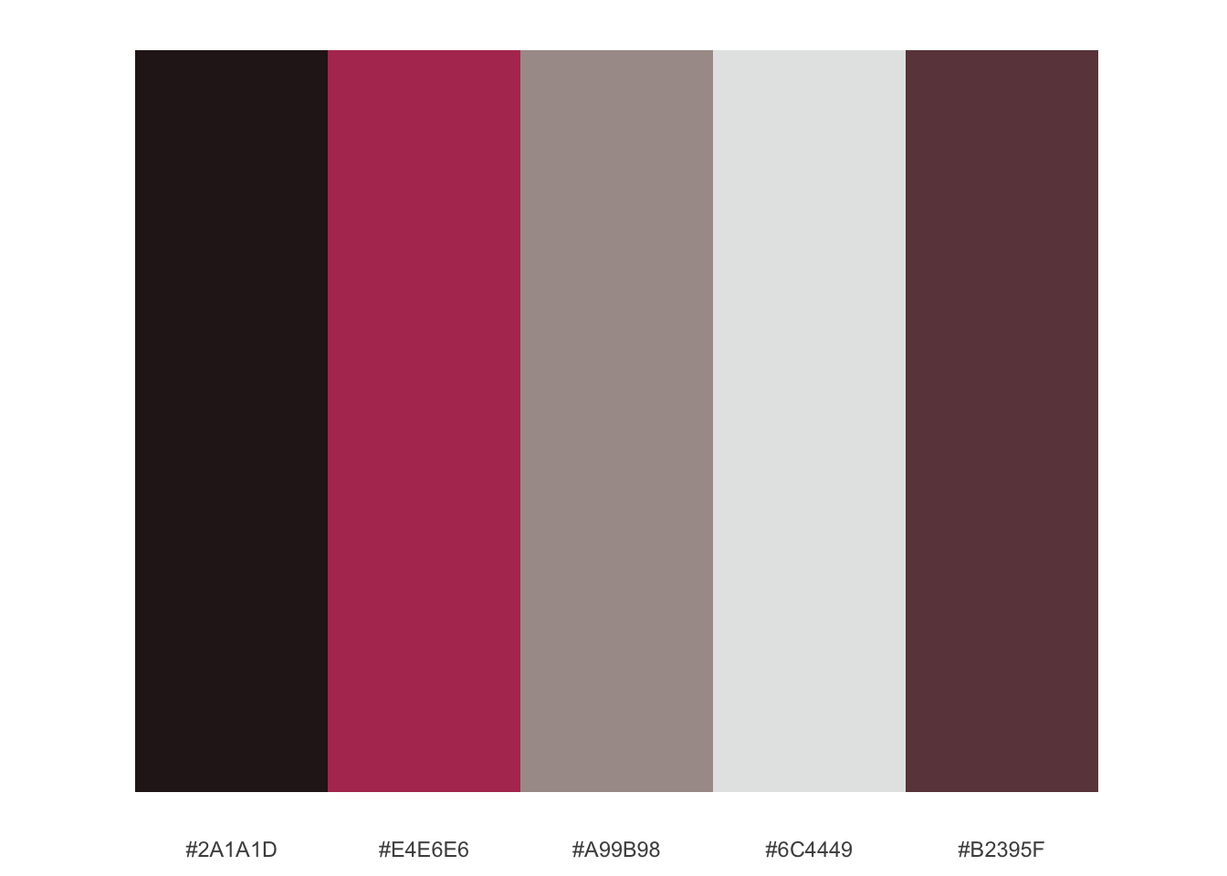
Which appears to be a more or less accurate representation of the colours in our image.

Concluding Remarks

As outlined above generating a colour palette from a arbitrary input image in R is pretty simple. The entire process should take no more than 10 seconds on a somewhat recent computer.

One could speed up the process probably quite significantly by re-sizing the image before reading it into R. It seems reasonable that results should not change too much even when halving the image’s dimensions. As we deal with two-dimensional data here, changes in image size will of course have an exponential effect on processing times.

Potentially one could take the output of the clustering (i.e. the palette) to generate a swatch for your favourite image editing software.

The code corresponding to this post can be found on my Gitlab.