Statistics, Science, Random Ramblings
A blog about data and other interesting things
Sirens in Düsseldorf
In this post, we are going to look at information about sirens in the city of Düsseldorf, Germany. These sirens are used to notify people in the city about dangers and hazards, usually in more severe events. Systems to provide warnings to the population in case of dangerous events have recently been subject to a lot of attention. This is due to the nationwide alert day which took place recently and was widely considered a failure as the systems often did not work as intended and many people never received any notification of some kind. Discussing this entire event and its implications is beyond the scope of this post, though.
The data we will be using is provided on the Open Data Düsseldorf site.
Namely we will use the file on the location of sirens and combine it with geodata of the city. Both data sets are available under the Data Licence Germany - Zero - 2.0.
There is a corresponding repository on my Gitlab.
So let’s get started.
Reading and cleaning the data
library("janitor")
library("sf")
library("tidyverse")
sirens <- read_delim("sirenen.csv",
locale = locale(decimal_mark = "."),
delim = ";")sirens <- clean_names(sirens)
glimpse(sirens)## Rows: 84
## Columns: 13
## $ latitude <dbl> 51.23091, 51.24676, 51.23448, 51.23146, 51.24399, …
## $ longitude <dbl> 6.706481, 6.727430, 6.752662, 6.727683, 6.738342, …
## $ altitude <dbl> 0, 0, 0, 0, 0, 0, 0, 0, 0, 0, 0, 0, 0, 0, 0, 0, 0,…
## $ geometry <chr> "point", "point", "point", "point", "point", "poin…
## $ nr <dbl> 1, 2, 3, 4, 5, 6, 7, 8, 9, 10, 11, 12, 13, 14, 15,…
## $ standort <chr> "Heerdter Landstraße 186", "Grevenbroicher Weg 70"…
## $ beschallungsradius <chr> "1200 Meter", "1100 Meter", "1000 Meter", "800 Met…
## $ stadtteil <chr> "Heerdt", "Lörick", "Oberkassel", "Heerdt", "Löric…
## $ stadtbezirksnummer <dbl> 4, 4, 4, 4, 4, 9, 10, 10, 10, 5, 5, 5, 6, 1, 1, 2,…
## $ stadtteilnummer <dbl> 42, 43, 41, 42, 43, 95, 101, 102, 102, 52, 51, 51,…
## $ plz <dbl> 40549, 40547, 40545, 40549, 40547, 40593, 40595, 4…
## $ utm_east <dbl> 32.33987, 32.34139, 32.34311, 32.34136, 32.34214, …
## $ utm_north <dbl> 5.678003, 5.679721, 5.678300, 5.678018, 5.679389, …The dataset is pretty clean, with one easily fixable issue. Each row represents a siren, there are 84 sirens in total.
The columns are as follows:
latitude,longitude: Coordinatesaltitude: Altitude, probably in m but see belowgeometry: Geometry type such as point, polygon, etc. but see belownr: Enumeration of the sirens (nr is short for Nummer, German for number)standort: street address (standort = place)beschallunsradius: radius of audibility (beschallungsradius = range of audibility)stadtteil: Name of city quarter the siren is in (stadtteil = quarter, 2nd administrative subdivision)stadtbezirksnummer: Number of the city’s borough (1st administrative subdivision)stadtteilnummer: Number of the city’s quarterplz: postal codeutm_east,utm_north: Coordinates in the UTM system
The one issue here is with the UTM columns, as the values are much too small. Fortunately we just need to shift the decimal dot a bit to fix this.
sirens <- sirens %>%
  mutate(utm_east = utm_east * 10e5,
         utm_north = utm_north * 10e5)
Let’s look at the missing values in the data:
sirens %>% map_int(function(x) sum(is.na(x)))## latitude longitude altitude geometry
## 0 0 0 0
## nr standort beschallungsradius stadtteil
## 0 0 5 0
## stadtbezirksnummer stadtteilnummer plz utm_east
## 0 0 0 0
## utm_north
## 0There are exactly five missings, which is quite good. They are all in the columns giving the audible range of the sirens, so we can either impute with the mean or to be on the more conservative side with the minimum.
Before we can do so, we need to remove the string part of the data in this column, as right now it looks like this:
head(sirens$beschallungsradius)## [1] "1200 Meter" "1100 Meter" "1000 Meter" "800 Meter" "600 Meter"
## [6] "1100 Meter"So, now we remove the string part and impute missings with the minimum.
sirens <- sirens %>%
    mutate(beschallungsradius = gsub(" Meter", "", .$beschallungsradius)) %>%
    mutate(beschallungsradius = as.numeric(.$beschallungsradius)) %>%
    replace_na(
        list(beschallungsradius = min(.$beschallungsradius, na.rm = TRUE)))
Next, let’s have a closer look at the altitude and geometry columns.
length(unique(sirens$geometry))## [1] 1length(unique(sirens$altitude))## [1] 1As it turns out both columns contain exactly one value.
sirens$geometry[1]## [1] "point"sirens$altitude[1]## [1] 0I guess it is safe to remove these variables from the data.
sirens <- sirens %>% select(-geometry, -altitude)Now we should proceed to prepare the data for plotting.
First, we read our geo data for the city. We use the version based on UTM-coordinates because these allow us to easily build circles around points using radii in metres.
dus <- st_read("stadtteile_etrs89.geojson")We retrieve the coordinate reference system from the geo data and use it to turn the sirens data into proper geo data. Without defining this we can not properly plot the data on top of each other.
sirens <- sirens %>%
  mutate(pt = map2(utm_east, utm_north, function(x, y) st_point(c(x, y)))) %>%
  st_sf(crs = st_crs(dus))
Based on the locations and the audible radii of the sirens we can now
construct the audible radii as geo data using st_buffer.
The data is slightly redundant as the buffer data also contains the locations
data, however as each sf object can only contain one active geometry we
need to have separate datasets.
buffer <- sirens %>%
  select(nr, beschallungsradius, pt) %>%
  mutate(radius = units::set_units(beschallungsradius, "m")) %>%
  mutate(geo_radius = st_buffer(pt, radius))

st_geometry(buffer) <- "geo_radius"
And as we now have prepared the data we are interested in, we can proceed with the plot. Plotting the data is fairly basic here.
ggplot() +
  geom_sf(data = dus, fill = "antiquewhite") +
  geom_sf(data = buffer, colour = "red", fill = "red", alpha = .3) +
  geom_sf(data = sirens, colour = "red") +
  coord_sf(datum = NA) +
  labs(title = "Sirens in Düsseldorf",
       subtitle = "Shown are sirens and their range of audibility",
       caption = "Data Source: Open Data Düsseldorf") +
  theme_minimal()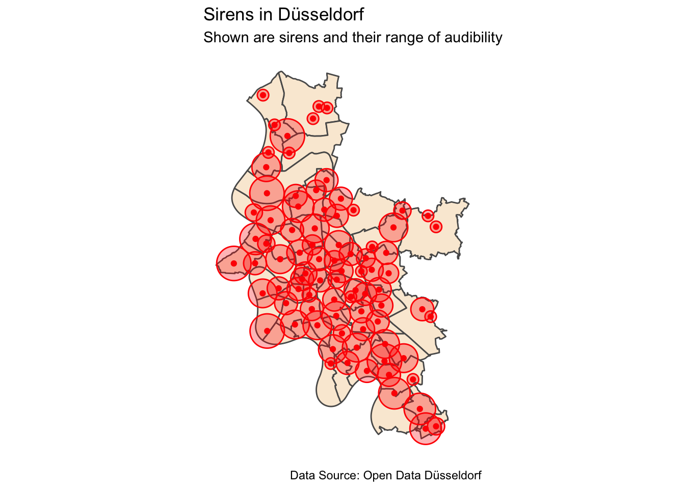
The map shows us that the 84 sirens in the city cover central parts fairly well. Some of the more remote areas of the city are more rural so the lack of coverage might not be as bad as it looks like in certain places; however the city’s administration should ensure that in case of emergencies everyone living in the city is in the range of audible alerts.
Unfortunately cell broadcasts for emergency warnings are not a thing in Germany yet. But even if they were, having sirens as a kind of low-tech fall-back seems like a good idea.
As for the dense coverage in the more central parts of the city it should be considered that noise levels are likely higher here compared to less central areas. Additionally there is most likely also a higher density of buildings which also might be larger than in the non-central parts of the city. This the nominal ranges of audibility for the sirens might not be reached under realistic circumstances, but there is no information on how these values were generated.