Fetching the data

So, let’s get started. First we load the required packages. The sf package is later needed to crop elements of the map.

library("dplyr")
library("ggplot2")
library("osmdata")
library("sf")

Then we can get the data from OSM. First, we need a bounding box to work with and then we can fetch the big streets.

# the bounding box, limiting what we fetch
location <- getbb("düsseldorf germany", featuretype = "city")

# the big streets
dus_streets <- location %>% 
  opq() %>% 
  add_osm_feature(key = "highway", 
                  value = c("motorway", "trunk",  "primary", 
                            "secondary", "tertiary")) %>% 
  osmdata_sf()

Depending on where you live you might want to have a look at the documentation to see what kind of elements you can return.

Next we fetch smaller streets. This can take a while and the object will require a lot of memory. Again, this might depend on what you visualise, but in my case that object is about 1GB.

small_streets <- location %>% 
  opq() %>% 
  add_osm_feature(
    key = "highway", 
    value = c("residential", "living", "unclassified", 
              "service", "footway")) %>% 
  osmdata_sf()

Next we can get the bodies of water in the city:

water <- location %>% 
  opq() %>% 
  add_osm_feature(key = "waterway", value = "river") %>% 
  osmdata_sf()

And now, as we are dealing with a city surrounded by even more cities we do also fetch the administrative boundaries of the cities within our bounding box. We can later fill the areas of neighbouring cities with the background colour of the plot to isolate the city we are interested in.

boundaries <- location %>%
  opq() %>%
  add_osm_feature(key = "admin_level", value = "6") %>%
  osmdata_sf()

An admin_level of 6 is what is appropriate for this region, but as always a look at the documentation should help you determine what you need for your map.

Plotting it

Before we can plot the data, some slight modifications have to be made. First, we create the background of the map, i.e. everything that is not Düsseldorf:

background <- boundaries$osm_multipolygons %>%
  filter(name != "Düsseldorf")

Each of the returned objects with OSM data includes a lot of data and you need to sort out which is the appropriate one to work on for each case:

boundaries

## Object of class 'osmdata' with:
##                  $bbox : 51.0654018,6.6163137,51.3854018,6.9363137
##         $overpass_call : The call submitted to the overpass API
##                  $meta : metadata including timestamp and version numbers
##            $osm_points : 'sf' Simple Features Collection with 20052 points
##             $osm_lines : 'sf' Simple Features Collection with 483 linestrings
##          $osm_polygons : 'sf' Simple Features Collection with 0 polygons
##        $osm_multilines : NULL
##     $osm_multipolygons : 'sf' Simple Features Collection with 11 multipolygons

The easiest way to find what you need is probably to just plot it.

Next, we split the water into the Rhine and everything else, enabling us to plot the Rhine in a different way than much smaller bodies of water. We also use st_crop from the sf package to cut the map data for the Rhine so it does not extend all the way to the plot’s borders.

small_water <- water$osm_lines %>%
  filter(name != "Rhein")

rhine <- water$osm_lines %>%
  filter(name == "Rhein") %>%
  st_crop(y = c(ymin = 51.12, ymax = 51.34, xmin = 6, xmax = 7))

Finally, we set the limits for the plot. Then we calculate the midpoint of the x-axis, which comes in handy when adding text to the plot and also we calculate the ratio of x to y which is very useful when determining the size of the plot when saving.

xlimit <- c(6.68, 6.95)
ylimit <- c(51.05, 51.36)
xmid <- xlimit[1] + diff(xlimit) / 2 
ratio <- diff(xlimit) / diff(ylimit)

And it is time to plot:

map <- ggplot() +
  # small streets
  geom_sf(data = small_streets$osm_lines, alpha = .6, 
          size = .2, colour = "grey30") +
  # large steets, making them stand out a bit with colour
  geom_sf(data = dus_streets$osm_lines, alpha = .8, 
          size = .4, colour = "goldenrod4") +
  # small water
  geom_sf(data = small_water, alpha = .8,
          size = .2, colour = "cadetblue") +
  # adding the background
  # need to increase size here, otherwise there will be a few semi-cutoff
  # streets directly at the city border
  geom_sf(data = background, colour = "grey10", size = 1.5, fill = "grey10") +
  # the rhine, have a large value for size so it stands out
  geom_sf(data = rhine, alpha = .8, size = 1.2, colour = "cadetblue") +
  # setting limits
  coord_sf(ylim = ylimit, xlim = xlimit, expand = FALSE) +
  # adding labels
  annotate(geom = "text", y = 51.085, x = xmid, 
           label = "Düsseldorf", size = 8, colour = "grey75",
           family = "PT Sans") +
  annotate(geom = "errorbarh", xmin = 6.72, xmax = 6.91, y = 51.075, height = 0,
           size = 0.5, colour = "grey50") +
  annotate(geom = "text", y = 51.07, x =  xmid,
           label = "51°13'32\"N  6°46'58\"E", family = "PT Sans", size = 3,
           colour = "grey50") +
  # finishing touches
  theme_void() +
  theme(panel.background = element_rect(fill = "grey10"),
        plot.background = element_rect(fill = "grey10"))

map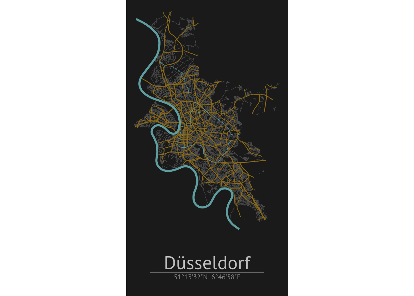

This looks nice, doesn’t it?

Finally, you can save the plot to disk, but you might have to adapt the sizes of the text beforehand – this is usually a bit of trial and error. Making use of the previously calculated ratio between the sides here gets the proportions about right (this might not work well for more extreme latitudes), but we also include the bg argument to avoid having any white borders in the plot.

ggsave("dus_map.png", map, height = 8, width = 8 * ratio, dpi = 300,
       bg = "grey10")

And this is it. Again, this post builds upon a tutorial from ggplot2tutor and is mainly an adaptation for more urban areas, I hope it is useful.

The map data is from OpenStreetMap (c) OpenStreetMap contributors, ODbL 1.0. https://www.openstreetmap.org/copyright